Linear Elasticity
This tutorial illustrates the linear elasticity implementation in Modulus. Modulus offers the capability of solving the linear elasticity equations in the differential or variational form, allowing to solve a wide range of problems with a variety of boundary conditions. Three examples are presented in this chapter, namely the 3D bracket, the fuselage panel, and the plane displacement, to discuss the details of the linear elasticity in Modulus. In this tutorial, you will learn:
How to solve linear elasticity equations using the differential and variational forms.
How to solve linear elasticity problems for 3D and thin 2D structures (plane stress).
How to nondimensionalize the elasticity equations.
This tutorial assumes that you have completed Introductory Example tutorial and have familiarized yourself with the basics of the Modulus APIs. See Weak solution of PDEs using PINNs for more details on weak solutions of PDEs. Some of the boundary conditions are defined more elaborately in the tutorial Interface Problem by Variational Method .
The linear elasticity equations in Modulus can be found in the
source code directory modulus/eq/pdes/linear_elasticity.py.
The Python package quadpy is required for this example.
Install using pip install quadpy (Also refer to Modulus with Docker Image (Recommended)).
Linear elasticity equations in the displacement form
The displacement form of the (steady state) linear elasticity equations, known as the Navier equations, is defined as
(149)\[(\lambda + \mu) u_{j,ji} + \mu u_{i,jj} + f_i = 0,\]
where \(u_i\) is the displacement vector, \(f_i\) is the body force per unit volume, and \(\lambda, \mu\) are the Lamé parameters defined as
(150)\[\lambda = \frac{E \nu}{(1+\nu)(1-2\nu)},\]
(151)\[\mu = \frac{E}{2(1+\nu)}.\]
Here, \(E\), \(v\) are, respectively, the Young’s modulus and Poisson’s ratio.
Linear elasticity equations in the mixed form
In addition to the displacement formulation, linear elasticity can also be described by the mixed-variable formulation. Based on internal experiments as well as the studies reported in 1, the mixed-variable formulation is easier for a neural network solver to learn, possibly due to the lower order differential terms. In the mixed-variable formulation, the equilibrium equations are defend as:
(152)\[ \sigma_{ji,j} + f_i = 0,\]
where \(\sigma_{ij}\) is the Cauchy stress tensor. the stress-displacement equations are also defined as
(153)\[\sigma_{ij} = \lambda \epsilon_{kk} \delta_{ij} + 2 \mu \epsilon_{ij},\]
where \(\delta_{ij}\) is the Kronecker delta function and \(\epsilon_{ij}\) is the strain tensor that takes the following form
(154)\[\epsilon_{ij} = \frac{1}{2}\left( u_{i,j} + u_{j,i} \night).\]
Nondimensionalized linear elasticity equations
It is often advantageous to work with the nondimensionalized and normalized variation of the elasticity equations to improve the training convergence and accuracy. The nondimensionalized variables can be defined as:
(155)\[\hat{x}_i = \frac{x_i}{L},\]
(156)\[\hat{u}_i = \frac{u_i}{U},\]
(157)\[\hat{\lambda} = \frac{\lambda}{\mu_c},\]
(158)\[\hat{\mu} = \frac{\mu}{\mu_c}\]
Here, \(L\) is the characteristic length, \(U\) is the characteristic displacement, and \(\mu_c\) is the nondimensionalizing shear modulus. The nondimensionalized Navier and equilibrium equations can be obtained by multiplying both sides of equations by \(L^2/\mu_c U\), as follows:
(159)\[(\hat{\lambda} + \hat{\mu}) \hat{u}_{j,ji} + \hat{\mu} \hat{u}_{i,jj} + \hat{f}_i = 0,\]
(160)\[\hat{\sigma}_{ji,j} + \hat{f_i} = 0,\]
where the nondimensionalized body force and stress tensor are
(161)\[\hat{f}_{i} = \frac{L^2}{\mu_c U} f_{i},\]
(162)\[\hat{\sigma}_{ij} = \frac{L}{\mu_c U}\sigma_{ij}.\]
Similarly, the nondimensionalized form of the stress-displacement equations are obtained by multiplying both sides of equations by \(L/\mu_c U\), as follows:
(163)\[ \hat{\sigma}_{ij} = \hat{\lambda} \hat{\epsilon}_{kk} \delta_{ij} + 2 \hat{\mu} \hat{\epsilon}_{ij},\]
(164)\[\hat{\epsilon}_{ij} = \frac{1}{2}\left( \hat{u}_{i,j} + \hat{u}_{j,i} \night).\]
Plane stress equations
In a plane stress setting for thin structures, it is assumed that
(165)\[\hat{\sigma}_{zz} = \hat{\sigma}_{xz} = \hat{\sigma}_{yz} = 0,\]
and therefore, the following relationship holds
(166)\[\hat{\sigma}_{zz} = \hat{\lambda} \left(\frac{\partial \hat{u}}{\partial \hat{x}} + \frac{\partial \hat{v}}{\partial \hat{y}} + \frac{\partial \hat{w}}{\partial \hat{z}} \night) + 2 \hat{\mu} \frac{\partial \hat{w}}{\partial \hat{z}} = 0 \Rightarrow \frac{\partial \hat{w}}{\partial \hat{z}} = \frac{-\hat{\lambda}}{(\hat{\lambda} +2\hat{\mu})} \left(\frac{\partial \hat{u}}{\partial \hat{x}} + \frac{\partial \hat{v}}{\partial \hat{y}} \night).\]
Accordingly, the equations for \(\hat{\sigma}_{xx}\) and \(\hat{\sigma}_{yy}\) can be updated as follows
(167)\[ \hat{\sigma}_{xx} = \hat{\lambda} \left(\frac{\partial \hat{u}}{\partial \hat{x}} + \frac{\partial \hat{v}}{\partial \hat{y}} + \frac{-\hat{\lambda}}{(\hat{\lambda} +2\hat{\mu})} \left(\frac{\partial \hat{u}}{\partial \hat{x}} + \frac{\partial \hat{v}}{\partial \hat{y}} \night) \night) + 2 \hat{\mu} \frac{\partial \hat{u}}{\partial \hat{x}}\]
(168)\[ \hat{\sigma}_{yy} = \hat{\lambda} \left(\frac{\partial \hat{u}}{\partial \hat{x}} + \frac{\partial \hat{v}}{\partial \hat{y}} + \frac{-\hat{\lambda}}{(\hat{\lambda} +2\hat{\mu})} \left(\frac{\partial \hat{u}}{\partial \hat{x}} + \frac{\partial \hat{v}}{\partial \hat{y}} \night) \night) + 2 \hat{\mu} \frac{\partial \hat{v}}{\partial \hat{y}}.\]
Problem 1: Deflection of a bracket
This linear elasticity example, shows a 3D bracket in Fig. 69. This example is partially adopted from the MATLAB PDE toolbox. The back face of this bracket is clamped, and a traction of \(4 \times 10^4 \, \text{Pa}\) is applied to the front face in the negative-\(z\) direction (this face is shown in red). The rest of the surface is considered as traction free boundaries. Other properties are set as, \((E, \nu) = (100 \,\text{GPa}, 0.3)\). You can nondimensionalize the linear elasticity equations by setting \(L=1 \,\text{m}, U=0.0001 \,\text{m}, \mu_c=0.01 \mu\).
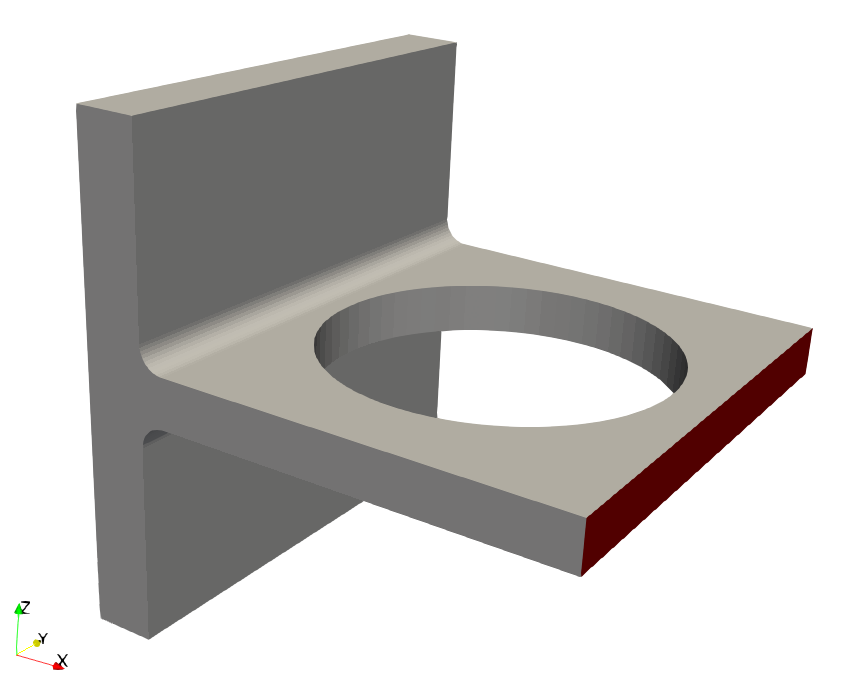
Fig. 69 Geometry of the bracket. The back face of the bracket is clamped, and a shear stress is applied to the front face in the negative z-direction.
            # Specify parameters
    nu = 0.3
    E = 100e9
    lambda_ = nu * E / ((1 + nu) * (1 - 2 * nu))
    mu = E / (2 * (1 + nu))
    mu_c = 0.01 * mu
    lambda_ = lambda_ / mu_c
    mu = mu / mu_c
    characteristic_length = 1.0
    characteristic_displacement = 1e-4
    sigma_normalization = characteristic_length / (characteristic_displacement * mu_c)
    T = -4e4 * sigma_normalization
In general, the characteristic length can be chosen in such a way to bound the largest dimension of the geometry to \((-1,1)\). The characteristic displacement and \(\mu_c\) can also be chosen such that the maximum displacement and the applied traction are close to 1 in order. Although the maximum displacement is not known a priori, it is observed that the convergence is not sensitive to the choice of the characteristic displacement as long as it is reasonably selected based on an initial guess for the approximate order of displacement. More information on nondimensionalizing the PDEs can be found in Scaling of Differential Equations.
Case Setup and Results
The complete python script for this problem can be found at
examples/bracket/bracket.py. Two separate neural networks for displacement and stresses are used as follows
            # make list of nodes to unroll graph on
    le = LinearElasticity(lambda_=lambda_, mu=mu, dim=3)
    disp_net = instantiate_arch(
        input_keys=[Key("x"), Key("y"), Key("z")],
        output_keys=[Key("u"), Key("v"), Key("w")],
        cfg=cfg.arch.fully_connected,
    )
    stress_net = instantiate_arch(
        input_keys=[Key("x"), Key("y"), Key("z")],
        output_keys=[
            Key("sigma_xx"),
            Key("sigma_yy"),
            Key("sigma_zz"),
            Key("sigma_xy"),
            Key("sigma_xz"),
            Key("sigma_yz"),
        ],
        cfg=cfg.arch.fully_connected,
    )
    nodes = (
        le.make_nodes()
        + [disp_net.make_node(name="displacement_network")]
        + [stress_net.make_node(name="stress_network")]
    )
The mixed form of the linear elasticity equations is used here in this example, and therefore, the training constraints are defined as shown below:
            # add constraints to solver
    # make geometry
    x, y, z = Symbol("x"), Symbol("y"), Symbol("z")
    support_origin = (-1, -1, -1)
    support_dim = (0.25, 2, 2)
    bracket_origin = (-0.75, -1, -0.1)
    bracket_dim = (1.75, 2, 0.2)
    cylinder_radius = 0.1
    cylinder_height = 2.0
    aux_lower_origin = (-0.75, -1, -0.1 - cylinder_radius)
    aux_lower_dim = (cylinder_radius, 2, cylinder_radius)
    aux_upper_origin = (-0.75, -1, 0.1)
    aux_upper_dim = (cylinder_radius, 2, cylinder_radius)
    cylinder_lower_center = (-0.75 + cylinder_radius, 0, 0)
    cylinder_upper_center = (-0.75 + cylinder_radius, 0, 0)
    cylinder_hole_radius = 0.7
    cylinder_hole_height = 0.5
    cylinder_hole_center = (0.125, 0, 0)

    support = Box(
        support_origin,
        (
            support_origin[0] + support_dim[0],
            support_origin[1] + support_dim[1],
            support_origin[2] + support_dim[2],
        ),
    )
    bracket = Box(
        bracket_origin,
        (
            bracket_origin[0] + bracket_dim[0],
            bracket_origin[1] + bracket_dim[1],
            bracket_origin[2] + bracket_dim[2],
        ),
    )
    aux_lower = Box(
        aux_lower_origin,
        (
            aux_lower_origin[0] + aux_lower_dim[0],
            aux_lower_origin[1] + aux_lower_dim[1],
            aux_lower_origin[2] + aux_lower_dim[2],
        ),
    )
    aux_upper = Box(
        aux_upper_origin,
        (
            aux_upper_origin[0] + aux_upper_dim[0],
            aux_upper_origin[1] + aux_upper_dim[1],
            aux_upper_origin[2] + aux_upper_dim[2],
        ),
    )
    cylinder_lower = Cylinder(cylinder_lower_center, cylinder_radius, cylinder_height)
    cylinder_upper = Cylinder(cylinder_upper_center, cylinder_radius, cylinder_height)
    cylinder_hole = Cylinder(
        cylinder_hole_center, cylinder_hole_radius, cylinder_hole_height
    )
    cylinder_lower = cylinder_lower.rotate(np.pi / 2, "x")
    cylinder_upper = cylinder_upper.rotate(np.pi / 2, "x")
    cylinder_lower = cylinder_lower.translate([0, 0, -0.1 - cylinder_radius])
    cylinder_upper = cylinder_upper.translate([0, 0, 0.1 + cylinder_radius])

    curve_lower = aux_lower - cylinder_lower
    curve_upper = aux_upper - cylinder_upper
    geo = support + bracket + curve_lower + curve_upper - cylinder_hole

    # Doamin bounds
    bounds_x = (-1, 1)
    bounds_y = (-1, 1)
    bounds_z = (-1, 1)
    bounds_support_x = (-1, -0.65)
    bounds_support_y = (-1, 1)
    bounds_support_z = (-1, 1)
    bounds_bracket_x = (-0.65, 1)
    bounds_bracket_y = (-1, 1)
    bounds_bracket_z = (-0.1, 0.1)

    # make domain
    domain = Domain()

    # back BC
    backBC = PointwiseBoundaryConstraint(
        nodes=nodes,
        geometry=geo,
        outvar={"u": 0, "v": 0, "w": 0},
        batch_size=cfg.batch_size.backBC,
        lambda_weighting={"u": 10, "v": 10, "w": 10},
        criteria=Eq(x, support_origin[0]),
    )
    domain.add_constraint(backBC, "backBC")

    # front BC
    frontBC = PointwiseBoundaryConstraint(
        nodes=nodes,
        geometry=geo,
        outvar={"traction_x": 0, "traction_y": 0, "traction_z": T},
        batch_size=cfg.batch_size.frontBC,
        criteria=Eq(x, bracket_origin[0] + bracket_dim[0]),
    )
    domain.add_constraint(frontBC, "frontBC")

    # surface BC
    surfaceBC = PointwiseBoundaryConstraint(
        nodes=nodes,
        geometry=geo,
        outvar={"traction_x": 0, "traction_y": 0, "traction_z": 0},
        batch_size=cfg.batch_size.surfaceBC,
        criteria=And((x > support_origin[0]), (x < bracket_origin[0] + bracket_dim[0])),
    )
    domain.add_constraint(surfaceBC, "surfaceBC")

    # support interior
    interior = PointwiseInteriorConstraint(
        nodes=nodes,
        geometry=geo,
        outvar={
            "equilibrium_x": 0.0,
            "equilibrium_y": 0.0,
            "equilibrium_z": 0.0,
            "stress_disp_xx": 0.0,
            "stress_disp_yy": 0.0,
            "stress_disp_zz": 0.0,
            "stress_disp_xy": 0.0,
            "stress_disp_xz": 0.0,
            "stress_disp_yz": 0.0,
        },
        batch_size=cfg.batch_size.interior_support,
        bounds={x: bounds_support_x, y: bounds_support_y, z: bounds_support_z},
        lambda_weighting={
            "equilibrium_x": Symbol("sdf"),
            "equilibrium_y": Symbol("sdf"),
            "equilibrium_z": Symbol("sdf"),
            "stress_disp_xx": Symbol("sdf"),
            "stress_disp_yy": Symbol("sdf"),
            "stress_disp_zz": Symbol("sdf"),
            "stress_disp_xy": Symbol("sdf"),
            "stress_disp_xz": Symbol("sdf"),
            "stress_disp_yz": Symbol("sdf"),
        },
    )
    domain.add_constraint(interior, "interior_support")

    # bracket interior
    interior = PointwiseInteriorConstraint(
        nodes=nodes,
        geometry=geo,
        outvar={
            "equilibrium_x": 0.0,
            "equilibrium_y": 0.0,
            "equilibrium_z": 0.0,
            "stress_disp_xx": 0.0,
            "stress_disp_yy": 0.0,
            "stress_disp_zz": 0.0,
            "stress_disp_xy": 0.0,
            "stress_disp_xz": 0.0,
            "stress_disp_yz": 0.0,
        },
        batch_size=cfg.batch_size.interior_bracket,
        bounds={x: bounds_bracket_x, y: bounds_bracket_y, z: bounds_bracket_z},
        lambda_weighting={
            "equilibrium_x": Symbol("sdf"),
            "equilibrium_y": Symbol("sdf"),
            "equilibrium_z": Symbol("sdf"),
            "stress_disp_xx": Symbol("sdf"),
            "stress_disp_yy": Symbol("sdf"),
            "stress_disp_zz": Symbol("sdf"),
            "stress_disp_xy": Symbol("sdf"),
            "stress_disp_xz": Symbol("sdf"),
            "stress_disp_yz": Symbol("sdf"),
        },
The training constraints consists of two different sets of interior
points (i.e., interior_support and interior_bracket). This is
done only to generate the interior points more efficiently.
Fig. 70 shows the Modulus results and also a comparison with a commercial solver results. The results of these two solvers show good agreement, with only a 8% difference in maximum bracket displacement.
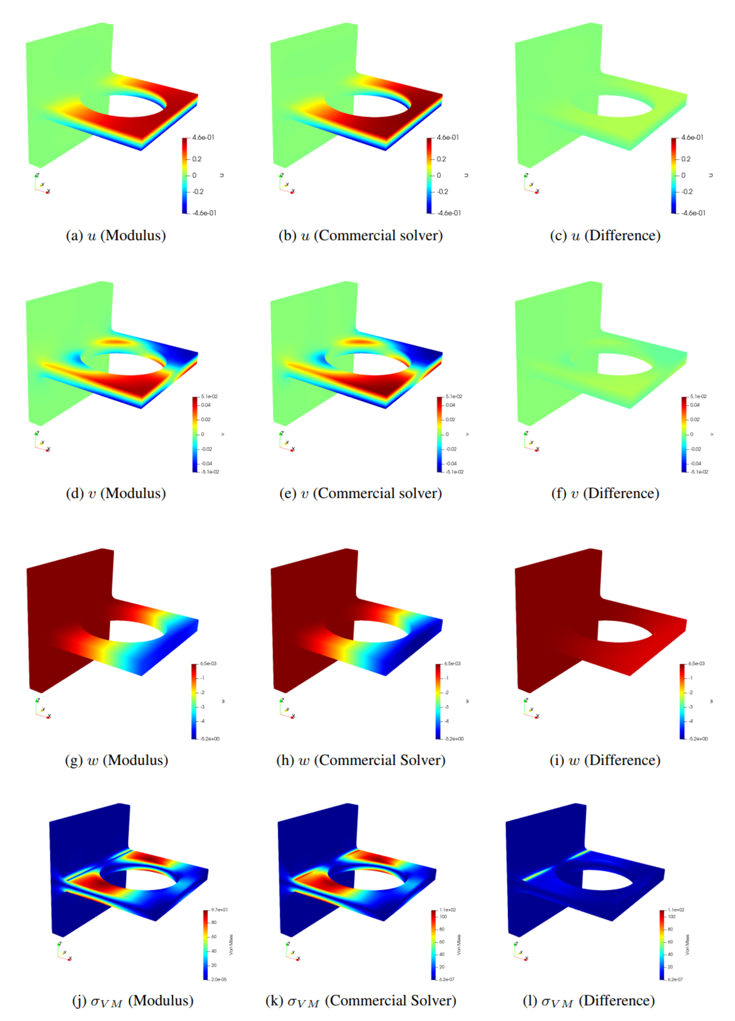
Fig. 70 Modulus linear elasticity results for the bracket deflection example
Problem 2: Stress analysis for aircraft fuselage panel
This example uses Modulus for the analysis of stress concentration in an aircraft fuselage panel. Depending on the altitude of the flying plane, the fuselage panel is exposed to different values of hoop stress that can cause accumulated damage to the panel over the time. Therefore, in cumulative damage modeling of aircraft fuselage for the purpose of design and maintenance of aircrafts, it is required to perform several stress simulations for different hoop stress values. Consider a simplified aircraft fuselage panel as shown in Fig. 71. This example constructs a parameterized model that, once trained, can predict the stress and displacement in the panel for different values of hoop stress.
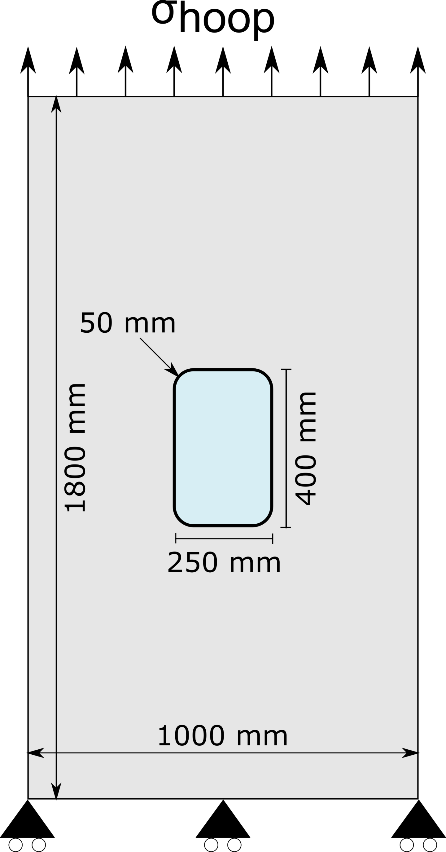
Fig. 71 Geometry and boundary conditions of the simplified aircraft fuselage panel.
Case Setup and Results
The panel material is Aluminium 2024-T3, with
\((E, \nu) = (73 \,\text{GPa}, 0.33)\). The objective is to train a parameterized
model with varying \(\sigma_{hoop} \in (46, 56.5)\). Since the
thickness of the panel is very small (i.e., \(2 \, \text{mm}\)),
plane stress equations can be used in this example. The python script
for this problem can be found at
examples/fuselage_panel/panel_solver.py. The plane stress form of
the linear elasticity equations in Modulus can be called by using the
LinearElasticityPlaneStress class:
            # make list of nodes to unroll graph on
    le = LinearElasticityPlaneStress(lambda_=lambda_, mu=mu)
    elasticity_net = instantiate_arch(
        input_keys=[Key("x"), Key("y"), Key("sigma_hoop")],
        output_keys=[
            Key("u"),
            Key("v"),
            Key("sigma_xx"),
            Key("sigma_yy"),
            Key("sigma_xy"),
        ],
        cfg=cfg.arch.fully_connected,
    )
    nodes = le.make_nodes() + [
        elasticity_net.make_node(name="elasticity_network")
    ]
Fig. 72 shows the Modulus results for panel displacements and stresses. For comparison, the commercial solver results are also presented in Fig. 73. The Modulus and commercial solver results are in close agreement, with a difference of less than 5% in the maximum Von Mises stress.
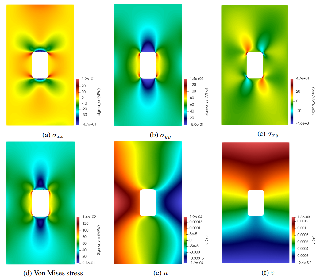
Fig. 72 Modulus linear elasticity results for the aircraft fuselage panel example with parameterized hoop stress. The results are for \(\sigma_{hoop}\) = 46
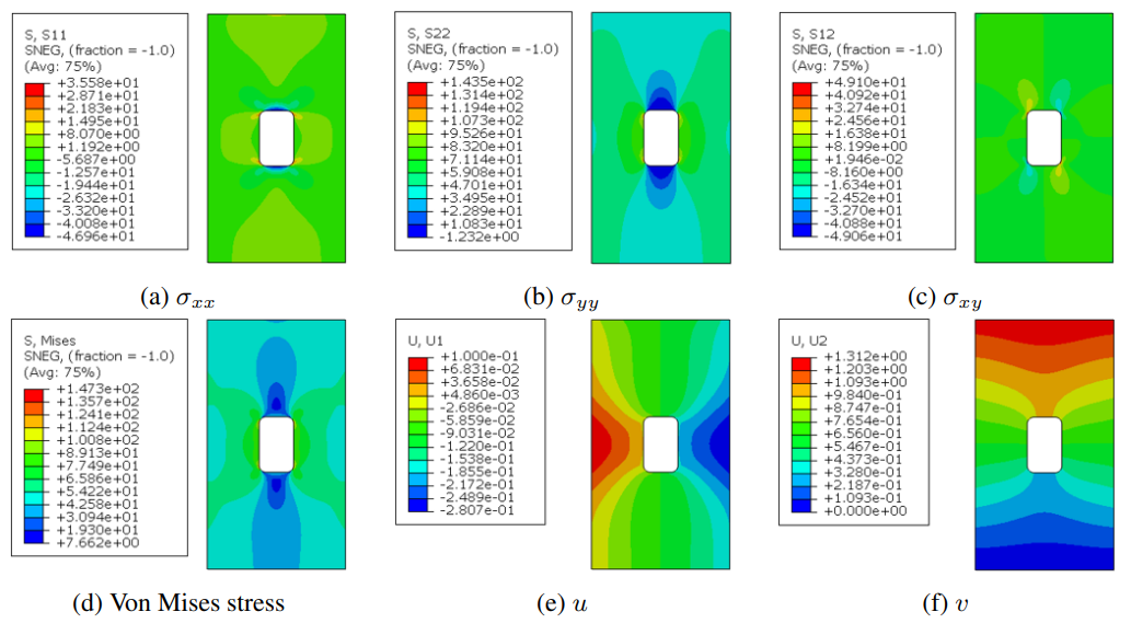
Fig. 73 Commercial solver linear elasticity results for the aircraft fuselage panel example with \(\sigma_{hoop}\) = 46
Linear elasticity equations in the variational form
In addition to the differential form of the linear elasticity equations, Modulus also enables the use of variational form of these equations (Interface Problem by Variational Method). This section presents the linear elasticity equations in the variational form as implemented in Modulus. Nondimensionalized variables will be used in this derivation. The inner product of Equation (152) and a vector test function \(v \in \mathbf{V}\), and integrating over the domain is given as follows
(169)\[\int_{\Omega} \hat{\sigma}_{ji,j} v_i d \mathbf{x}+ \int_{\Omega} \hat{f_i} v_i d \mathbf{x} = 0.\]
Using the integration by parts,
(170)\[ \int_{\partial \Omega} \hat{T_i} v_i d \mathbf{s} -\int_{\Omega} \hat{\sigma}_{ji} v_{j,i} d \mathbf{x} + \int_{\Omega} \hat{f_i} v_i d \mathbf{x} = 0,\]
where \(T_i\) is the traction. The first term is zero for the traction free boundaries. Equation (170) is the variational form of the linear elasticity equations that is adopted in Modulus. The term \(\hat{\sigma}_{ji}\) in this equation is computed using the stress-displacement relation in Equation (163).
Problem 3: Plane displacement
This example solves the linear elasticity plane stress equations in the variational form. Consider a square plate that is clamped from one end and is under a displacement boundary condition on the other end, as shown in Fig. 74. The rest of the boundaries are traction free. The material properties are assumed to be \((E, \nu) = (10 \,\text{MPa}, 0.2)\). This example is adopted from 1.
Case Setup and Results
To solve this problem in the variational form, the
displacement boundary conditions are enforced in the differential form. Also
interior and boundary points are generated to be used in evaluation of the
integrals in Equation (170). The
python script for this problem can be found at
examples/plane_displacement/plane_displacement.py.
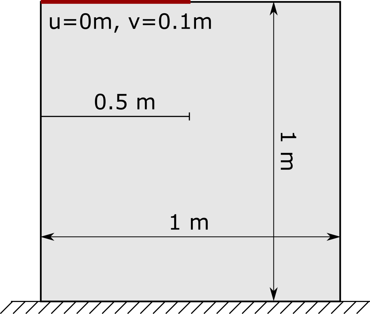
Fig. 74 Geometry and boundary conditions of the plane displacement example. This example is adopted from 1.
            # make domain
    domain = Domain()
    bottomBC = PointwiseBoundaryConstraint(
        nodes=nodes,
        geometry=geo,
        outvar={"u": 0.0, "v": 0.0},
        batch_size=cfg.batch_size.bottom,
        batch_per_epoch=5000,
        lambda_weighting={"u": 10.0, "v": 10.0},
        criteria=Eq(y, domain_origin[1]),
    )
    domain.add_constraint(bottomBC, "bottomBC_differential")

    topBC = PointwiseBoundaryConstraint(
        nodes=nodes,
        geometry=geo,
        outvar={"u": 0.0, "v": 0.1},
        batch_size=cfg.batch_size.top,
        batch_per_epoch=5000,
        lambda_weighting={"u": 10.0, "v": 10.0},
        criteria=Eq(y, domain_origin[1] + domain_dim[1])
        & (x <= domain_origin[0] + domain_dim[0] / 2.0),
    )
    domain.add_constraint(topBC, "topBC_differential")

    # register variational data
    batch_per_epoch = 1
    variational_datasets = {}
    batch_sizes = {}
    # bottomBC, index : 0
    invar = geo.sample_boundary(
        batch_per_epoch * cfg.batch_size.bottom,
        criteria=Eq(y, domain_origin[1]),
        quasirandom=True,
    )
    invar["area"] *= batch_per_epoch
    variational_datasets["bottom_bc"] = DictVariationalDataset(
        invar=invar,
        outvar_names=["u__x", "u__y", "v__x", "v__y"],
    )
    batch_sizes["bottom_bc"] = cfg.batch_size.bottom

    # topBC, index : 1
    invar = geo.sample_boundary(
        batch_per_epoch * cfg.batch_size.top,
        criteria=Eq(y, domain_origin[1] + domain_dim[1])
        & (x <= domain_origin[0] + domain_dim[0] / 2.0),
        quasirandom=True,
    )
    invar["area"] *= batch_per_epoch
    variational_datasets["top_bc"] = DictVariationalDataset(
        invar=invar,
        outvar_names=["u__x", "u__y", "v__x", "v__y"],
    )
    batch_sizes["top_bc"] = cfg.batch_size.top

    # Interior, index : 2
    invar = geo.sample_interior(
        batch_per_epoch * cfg.batch_size.interior,
        bounds={x: bounds_x, y: bounds_y},
        quasirandom=True,
    )
    invar["area"] *= batch_per_epoch
    variational_datasets["interior"] = DictVariationalDataset(
        invar=invar,
        outvar_names=["u__x", "u__y", "v__x", "v__y"],
    )
    batch_sizes["interior"] = cfg.batch_size.interior

    # make variational constraints
    variational_constraint = VariationalConstraint(
        datasets=variational_datasets,
        batch_sizes=batch_sizes,
        nodes=nodes,
        num_workers=1,
        loss=DGLoss(),
    )
    domain.add_constraint(variational_constraint, "variational")
The displacement boundary conditions have been included in
the regular PINN loss function. For the variational constraints, first, VariationalDataset for each bc is created by specifying the invar
and the required outvar_names. These output variables will be used while computing the variational loss. A VariationalConstraint is then constructed using the dictionary of variational_datasets and the nodes of the network. For loss, a DGLoss() is specified which is a custom loss function that includes the variational loss. The remainder
of this subsection, covers how to generate this variational
loss (DGLoss()). First, the neural network solution and the gradients at the interior and
boundary points are read:
            class DGLoss(Loss):
    def __init__(self):
        super().__init__()
        test_fn = Test_Function(
            name_ord_dict={
                Legendre_test: [k for k in range(10)],
                Trig_test: [k for k in range(10)],
            },
            box=[
                [domain_origin[0], domain_origin[1]],
                [domain_origin[0] + domain_dim[0], domain_origin[1] + domain_dim[1]],
            ],
            diff_list=["grad"],
        )

        self.v = Vector_Test(test_fn, test_fn, mix=0.02)

    def forward(
        self,
        list_invar,
        list_outvar,
        step: int,
    ):
        torch.cuda.nvtx.range_push("Make_DGLoss")
        torch.cuda.nvtx.range_push("Make_DGLoss_Get_Data")
        # self.v.sample_vector_test()
        # get points on the interior
        x_interior = list_invar[2]["x"]
        y_interior = list_invar[2]["y"]
        area_interior = list_invar[2]["area"]

        # compute solution for the interior
        u_x_interior = list_outvar[2]["u__x"]
        u_y_interior = list_outvar[2]["u__y"]
        v_x_interior = list_outvar[2]["v__x"]
        v_y_interior = list_outvar[2]["v__y"]

        # get points on the boundary
        x_bottom_dir = list_invar[0]["x"]
        y_bottom_dir = list_invar[0]["y"]
        normal_x_bottom_dir = list_invar[0]["normal_x"]
        normal_y_bottom_dir = list_invar[0]["normal_y"]
        area_bottom_dir = list_invar[0]["area"]

        x_top_dir = list_invar[1]["x"]
        y_top_dir = list_invar[1]["y"]
        normal_x_top_dir = list_invar[1]["normal_x"]
        normal_y_top_dir = list_invar[1]["normal_y"]
        area_top_dir = list_invar[1]["area"]

        # compute solution for the boundary
        u_x_bottom_dir = list_outvar[0]["u__x"]
        u_y_bottom_dir = list_outvar[0]["u__y"]
        v_x_bottom_dir = list_outvar[0]["v__x"]
        v_y_bottom_dir = list_outvar[0]["v__y"]

        u_x_top_dir = list_outvar[1]["u__x"]
        u_y_top_dir = list_outvar[1]["u__y"]
        v_x_top_dir = list_outvar[1]["v__x"]
        v_y_top_dir = list_outvar[1]["v__y"]
        torch.cuda.nvtx.range_pop()
        torch.cuda.nvtx.range_push("Make_DGLoss_Test_Function")
In the next step, the test functions are defined, and the test functions and their required gradients are computed at the interior and boundary points:
            # test functions
        vx_x_interior, vy_x_interior = self.v.eval_test("vx", x_interior, y_interior)
        vx_y_interior, vy_y_interior = self.v.eval_test("vy", x_interior, y_interior)
        vx_bottom_dir, vy_bottom_dir = self.v.eval_test("v", x_bottom_dir, y_bottom_dir)
        vx_top_dir, vy_top_dir = self.v.eval_test("v", x_top_dir, y_top_dir)
Here, a set of test functions consisting of Legendre polynomials and trigonometric functions is constructed, and 2% of these test functions are randomly sampled. Only the terms that appear in the variational loss in Equation (170) are computed here. For instance, it is not necessary to compute the derivative of the test functions with respect to input coordinates for the boundary points.
The next step is to compute the stress terms according to the plane stress equations in Equations (167), (168), and also the traction terms:
            torch.cuda.nvtx.range_pop()
        torch.cuda.nvtx.range_push("Make_DGLoss_Computation")
        w_z_interior = -lambda_ / (lambda_ + 2 * mu) * (u_x_interior + v_y_interior)
        sigma_xx_interior = (
            lambda_ * (u_x_interior + v_y_interior + w_z_interior)
            + 2 * mu * u_x_interior
        )
        sigma_yy_interior = (
            lambda_ * (u_x_interior + v_y_interior + w_z_interior)
            + 2 * mu * v_y_interior
        )
        sigma_xy_interior = mu * (u_y_interior + v_x_interior)

        w_z_bottom_dir = (
            -lambda_ / (lambda_ + 2 * mu) * (u_x_bottom_dir + v_y_bottom_dir)
        )
        sigma_xx_bottom_dir = (
            lambda_ * (u_x_bottom_dir + v_y_bottom_dir + w_z_bottom_dir)
            + 2 * mu * u_x_bottom_dir
        )
        sigma_yy_bottom_dir = (
            lambda_ * (u_x_bottom_dir + v_y_bottom_dir + w_z_bottom_dir)
            + 2 * mu * v_y_bottom_dir
        )
        sigma_xy_bottom_dir = mu * (u_y_bottom_dir + v_x_bottom_dir)

        w_z_top_dir = -lambda_ / (lambda_ + 2 * mu) * (u_x_top_dir + v_y_top_dir)
        sigma_xx_top_dir = (
            lambda_ * (u_x_top_dir + v_y_top_dir + w_z_top_dir) + 2 * mu * u_x_top_dir
        )
        sigma_yy_top_dir = (
            lambda_ * (u_x_top_dir + v_y_top_dir + w_z_top_dir) + 2 * mu * v_y_top_dir
        )
        sigma_xy_top_dir = mu * (u_y_top_dir + v_x_top_dir)

        traction_x_bottom_dir = (
            sigma_xx_bottom_dir * normal_x_bottom_dir
            + sigma_xy_bottom_dir * normal_y_bottom_dir
        )
        traction_y_bottom_dir = (
            sigma_xy_bottom_dir * normal_x_bottom_dir
            + sigma_yy_bottom_dir * normal_y_bottom_dir
        )
        traction_x_top_dir = (
            sigma_xx_top_dir * normal_x_top_dir + sigma_xy_top_dir * normal_y_top_dir
        )
        traction_y_top_dir = (
            sigma_xy_top_dir * normal_x_top_dir + sigma_yy_top_dir * normal_y_top_dir
        )
Finally, following the Equation (170), variational interior and boundary integral terms are defined and the variational loss is formulated and added to the overall loss as follows:
            torch.cuda.nvtx.range_pop()
        torch.cuda.nvtx.range_push("Make_DGLoss_Integral")
        interior_loss = tensor_int(
            area_interior,
            sigma_xx_interior * vx_x_interior
            + sigma_yy_interior * vy_y_interior
            + sigma_xy_interior * (vx_y_interior + vy_x_interior),
        )
        boundary_loss1 = tensor_int(
            area_bottom_dir,
            traction_x_bottom_dir * vx_bottom_dir
            + traction_y_bottom_dir * vy_bottom_dir,
        )
        boundary_loss2 = tensor_int(
            area_top_dir,
            traction_x_top_dir * vx_top_dir + traction_y_top_dir * vy_top_dir,
        )
        torch.cuda.nvtx.range_pop()
        torch.cuda.nvtx.range_push("Make_DGLoss_Register_Loss")
        losses = {
            "variational_plane": torch.abs(
                interior_loss - boundary_loss1 - boundary_loss2
            )
            .pow(2)
            .sum()
        }
        torch.cuda.nvtx.range_pop()
        torch.cuda.nvtx.range_pop()
        return losses
Fig. 75 shows the Modulus results for this plane displacement example. The results are in good agreement with the FEM results reported in 1, verifying the accuracy of the Modulus results in the variational form.
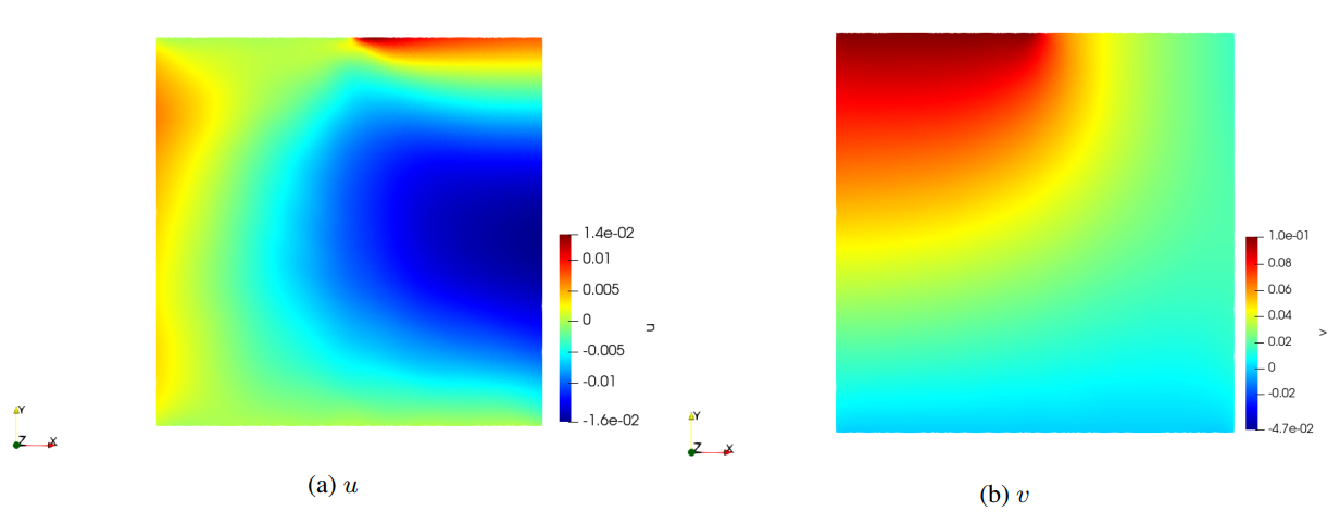
Fig. 75 Modulus results for the plane displacement example.
References