Geometry Modules
Modulus provides several 1D, 2D and 3D primitives that can be used for sampling point clouds required for the physics-informed training.
These primitives support the standard boolean operations* like Union (+ ), Intersection (& ) and Subtraction (- ). The boolean
operations work on the signed distance fields of the differnt primitives.
Below example shows a simple CSG primitive being built using Modulus.
Listing 1 Constructive solid geometry
            import numpy as np
from modulus.geometry.primitives_3d import Box, Sphere, Cylinder
from modulus.utils.io.vtk import var_to_polyvtk

# number of points to sample
nr_points = 100000

# make standard constructive solid geometry example
# make primitives
box = Box(point_1=(-1, -1, -1), point_2=(1, 1, 1))
sphere = Sphere(center=(0, 0, 0), radius=1.2)
cylinder_1 = Cylinder(center=(0, 0, 0), radius=0.5, height=2)
cylinder_2 = cylinder_1.rotate(angle=float(np.pi / 2.0), axis="x")
cylinder_3 = cylinder_1.rotate(angle=float(np.pi / 2.0), axis="y")

# combine with boolean operations
all_cylinders = cylinder_1 + cylinder_2 + cylinder_3
box_minus_sphere = box & sphere
geo = box_minus_sphere - all_cylinders

# sample geometry for plotting in Paraview
s = geo.sample_boundary(nr_points=nr_points)
var_to_polyvtk(s, "boundary")
print("Surface Area:{:.3f}".format(np.sum(s["area"])))
s = geo.sample_interior(nr_points=nr_points, compute_sdf_derivatives=True)
var_to_polyvtk(s, "interior")
print("Volume:{:.3f}".format(np.sum(s["area"])))
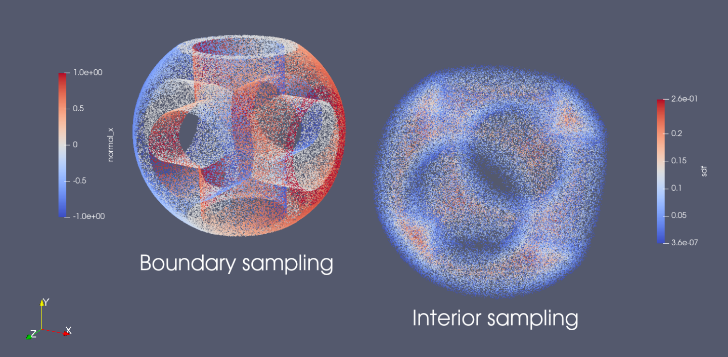
Fig. 33 Constructive Solid Geometry using Modulus primitives
A complete list of primitives can be referred in modulus.geometry.primitives_*
While generating a complex primitive, it should be noted that the boolean operation are performed at the final stage, meaning it is invariant to the order of the boolean operations. In other words, if you are subtracting a primitive from another primitive, and if you decide to add a different primitive in the area that is subtracted, you will not see the newly added primitive because the subtracted primitive.
The geometry objects created also support operations like translate, scale, rotate and repeat to further generate more complicated primitives
Listing 2 Transforms and Repeat
            # apply transformations
geo = geo.scale(0.5)
geo = geo.rotate(angle=np.pi / 4, axis="z")
geo = geo.rotate(angle=np.pi / 4, axis="y")
geo = geo.repeat(spacing=4.0, repeat_lower=(-1, -1, -1), repeat_higher=(1, 1, 1))

# sample geometry for plotting in Paraview
s = geo.sample_boundary(nr_points=nr_points)
var_to_polyvtk(s, "repeated_boundary")
print("Repeated Surface Area:{:.3f}".format(np.sum(s["area"])))
s = geo.sample_interior(nr_points=nr_points, compute_sdf_derivatives=True)
var_to_polyvtk(s, "repeated_interior")
print("Repeated Volume:{:.3f}".format(np.sum(s["area"])))
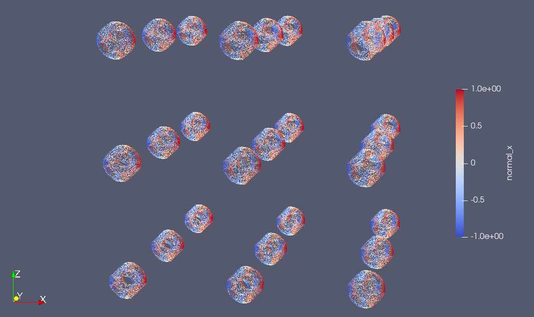
Fig. 34 Geometry transforms
The CSG objects can be easily parameterized using sympy. An example of this is used in Parameterized 3D Heat Sink
Listing 3 Parameterized geometry
            from modulus.geometry.primitives_2d import Rectangle, Circle
from modulus.utils.io.vtk import var_to_polyvtk
from modulus.geometry.parameterization import Parameterization, Parameter

# make plate with parameterized hole
# make parameterized primitives
plate = Rectangle(point_1=(-1, -1), point_2=(1, 1))
y_pos = Parameter("y_pos")
parameterization = Parameterization({y_pos: (-1, 1)})
circle = Circle(center=(0, y_pos), radius=0.3, parameterization=parameterization)
geo = plate - circle

# sample geometry over entire parameter range
s = geo.sample_boundary(nr_points=100000)
var_to_polyvtk(s, "parameterized_boundary")
s = geo.sample_interior(nr_points=100000)
var_to_polyvtk(s, "parameterized_interior")

# sample specific parameter
s = geo.sample_boundary(
    nr_points=100000, parameterization=Parameterization({y_pos: 0})
)
var_to_polyvtk(s, "y_pos_zero_boundary")
s = geo.sample_interior(
    nr_points=100000, parameterization=Parameterization({y_pos: 0})
)
var_to_polyvtk(s, "y_pos_zero_interior")
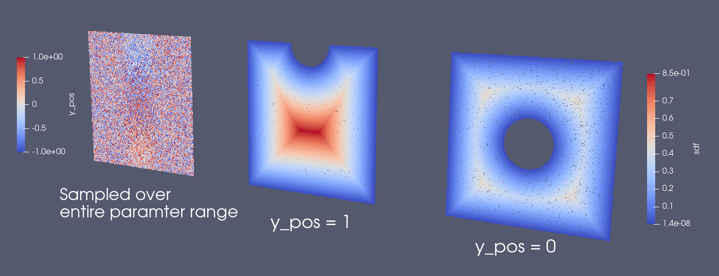
Fig. 35 Parameterized Constructive Solid Geometry using Modulus primitives
Some interesting shapes generated using Modulus’ geometry module are presented below
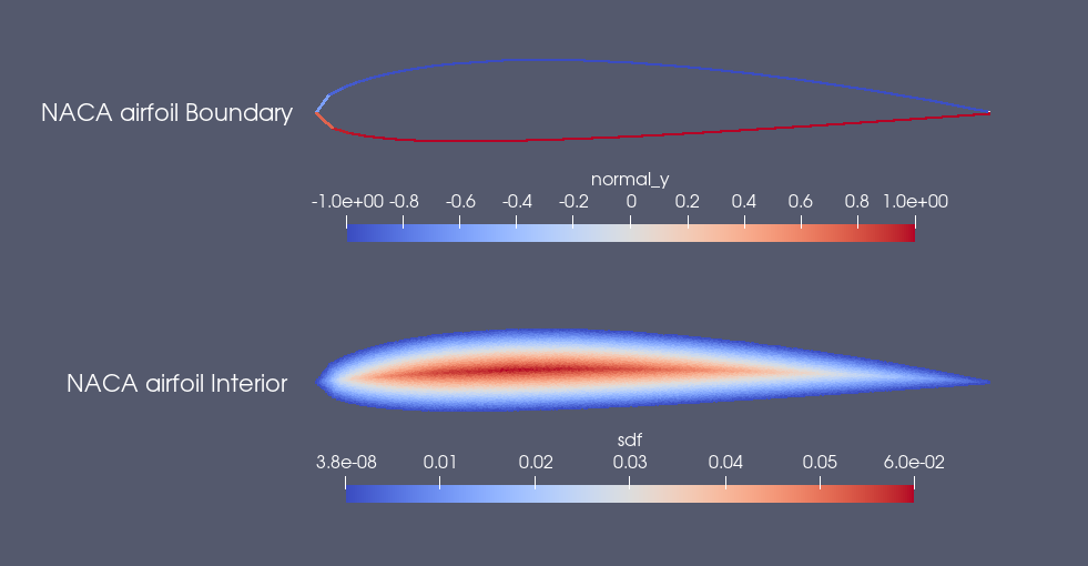
Fig. 36 NACA airfoil using
Polygon primitive. (script at
/examples/geometry/naca_airfoil.py)
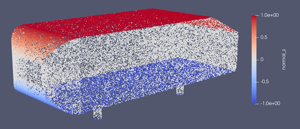
Fig. 37 Ahmed body
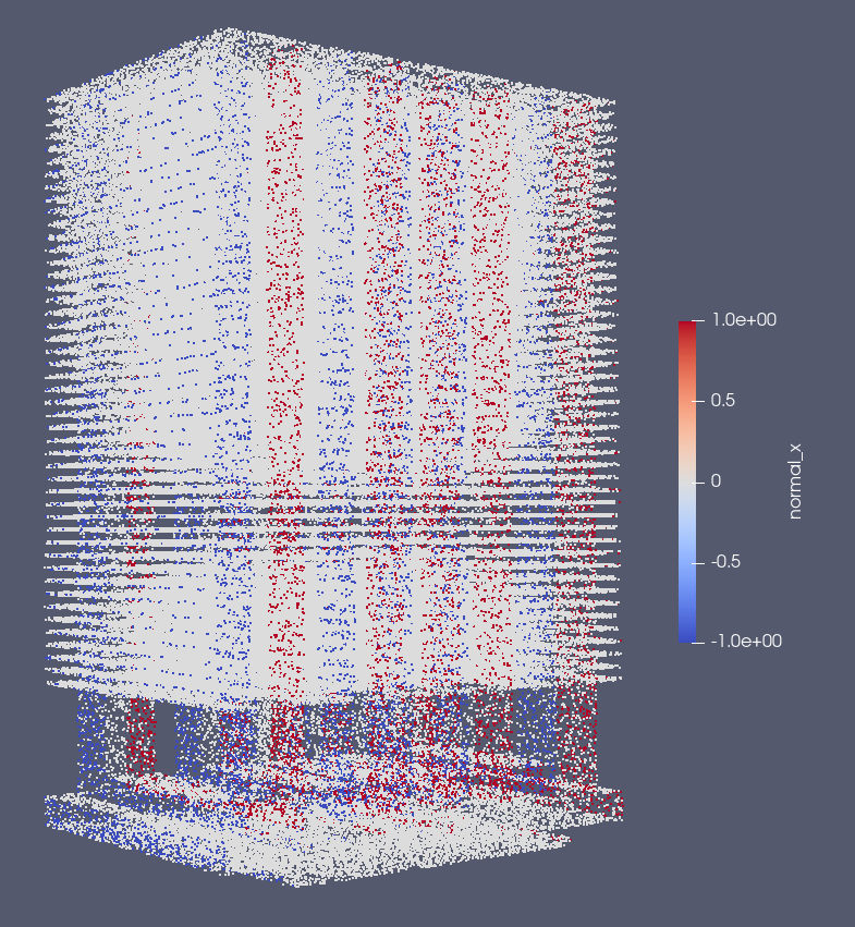
Fig. 38 Industrial heatsink geometry
If you don’t find a primitive defined for your application, it is easy to setup using the base classes from Modulus. All you need to do is come up with and appropriate expression for the signed distance field and the surfaces of the geometry. An example is shown below.
Listing 4 Custom Primitive
            from sympy import Symbol, pi, sin, cos, sqrt, Min, Max, Abs

from modulus.geometry.geometry import Geometry, csg_curve_naming
from modulus.geometry.helper import _sympy_sdf_to_sdf
from modulus.geometry.curve import SympyCurve, Curve
from modulus.geometry.parameterization import Parameterization, Parameter, Bounds
from modulus.geometry.primitives_3d import Cylinder
from modulus.utils.io.vtk import var_to_polyvtk

class InfiniteCylinder(Geometry):
    """
3D Infinite Cylinder
Axis parallel to z-axis, no caps on ends

Parameters
----------
center : tuple with 3 ints or floats
center of cylinder
radius : int or float
radius of cylinder
height : int or float
height of cylinder
parameterization : Parameterization
Parameterization of geometry.
"""

    def __init__(self, center, radius, height, parameterization=Parameterization()):
        # make sympy symbols to use
        x, y, z = Symbol("x"), Symbol("y"), Symbol("z")
        h, r = Symbol(csg_curve_naming(0)), Symbol(csg_curve_naming(1))
        theta = Symbol(csg_curve_naming(2))

        # surface of the cylinder
        curve_parameterization = Parameterization(
            {h: (-1, 1), r: (0, 1), theta: (0, 2 * pi)}
        )
        curve_parameterization = Parameterization.combine(
            curve_parameterization, parameterization
        )
        curve_1 = SympyCurve(
            functions={
                "x": center[0] + radius * cos(theta),
                "y": center[1] + radius * sin(theta),
                "z": center[2] + 0.5 * h * height,
                "normal_x": 1 * cos(theta),
                "normal_y": 1 * sin(theta),
                "normal_z": 0,
            },
            parameterization=curve_parameterization,
            area=height * 2 * pi * radius,
        )
        curves = [curve_1]

        # calculate SDF
        r_dist = sqrt((x - center[0]) ** 2 + (y - center[1]) ** 2)
        sdf = radius - r_dist

        # calculate bounds
        bounds = Bounds(
            {
                Parameter("x"): (center[0] - radius, center[0] + radius),
                Parameter("y"): (center[1] - radius, center[1] + radius),
                Parameter("z"): (center[2] - height / 2, center[2] + height / 2),
            },
            parameterization=parameterization,
        )

        # initialize Infinite Cylinder
        super().__init__(
            curves,
            _sympy_sdf_to_sdf(sdf),
            dims=3,
            bounds=bounds,
            parameterization=parameterization,
        )


nr_points = 100000

cylinder_1 = Cylinder(center=(0, 0, 0), radius=0.5, height=2)
cylinder_2 = InfiniteCylinder(center=(0, 0, 0), radius=0.5, height=2)

s = cylinder_1.sample_interior(nr_points=nr_points, compute_sdf_derivatives=True)
var_to_polyvtk(s, "interior_cylinder")

s = cylinder_2.sample_interior(nr_points=nr_points, compute_sdf_derivatives=True)
var_to_polyvtk(s, "interior_infinite_cylinder")
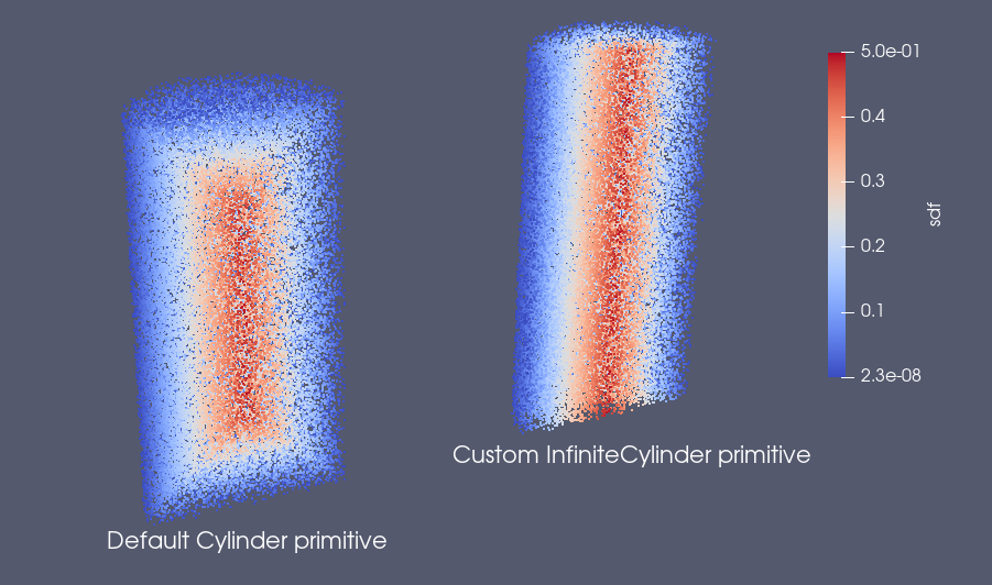
Fig. 39 Custom primitive in Modulus. The cylinders are sliced to visualize the interior SDF
For more complicated shapes, Modulus allows geometries to be imported in the STL format. The module uses ray tracing to compute SDF and its derivatives. The module also gives surface normals of the geometry for surface sampling. Once the geometry is imported, the point cloud can be used for training. An example of this can be found in STL Geometry: Blood Flow in Intracranial Aneurysm.
Tesselated geometries can also be combined with the primitives
Listing 5 Tesselated Geometry
            import numpy as np
from modulus.geometry.tessellation import Tessellation
from modulus.geometry.primitives_3d import Plane
from modulus.utils.io.vtk import var_to_polyvtk

# number of points to sample
nr_points = 100000

# make tesselated geometry from stl file
geo = Tessellation.from_stl("./stl_files/tessellated_example.stl")

# tesselated geometries can be combined with primitives
cut_plane = Plane((0, -1, -1), (0, 1, 1))
geo = geo & cut_plane

# sample geometry for plotting in Paraview
s = geo.sample_boundary(nr_points=nr_points)
var_to_polyvtk(s, "tessellated_boundary")
print("Repeated Surface Area:{:.3f}".format(np.sum(s["area"])))
s = geo.sample_interior(nr_points=nr_points, compute_sdf_derivatives=True)
var_to_polyvtk(s, "tessellated_interior")
print("Repeated Volume:{:.3f}".format(np.sum(s["area"])))
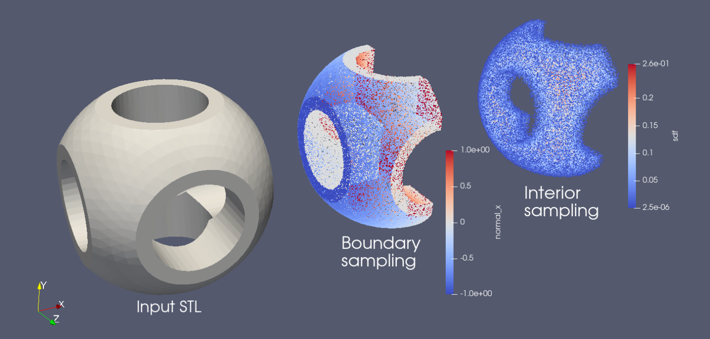
Fig. 40 Tesselated Geometry sampling using Modulus
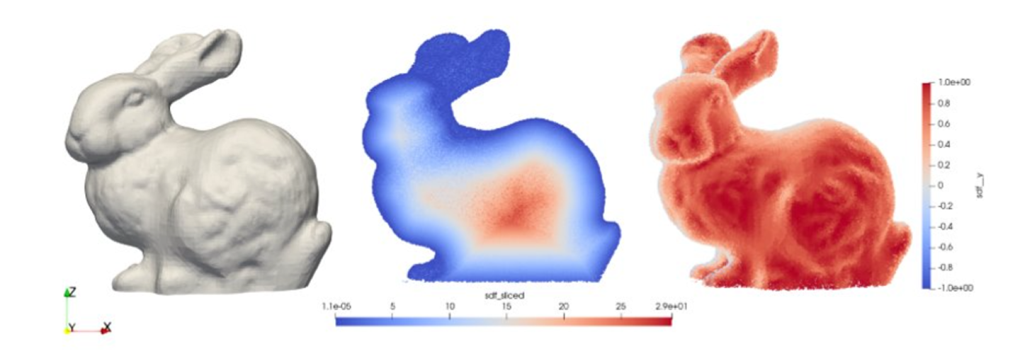
Fig. 41 Tesselated Geometry sampling using Modulus: Stanford bunny