Coupled Spring Mass ODE System
In this tutorial Modulus is used to solve a system of coupled ordinary differential equations. Since the APIs used for this problem have already been covered in a previous tutorial, only the problem description is discussed without going into the details of the code.
This tutorial assumes that you have completed tutorial Introductory Example and have familiarized yourself with the basics of the Modulus APIs. Also, refer to tutorial 1D Wave Equation for information on defining new differential equations, and solving time dependent problems in Modulus.
In this tutorial, a simple spring mass system as shown in Fig. 63 is solved. The systems shows three masses attached to each other by four springs. The springs slide along a frictionless horizontal surface. The masses are assumed to be point masses and the springs are massless. The problem is solved so that the masses (\(m's\)) and the spring constants (\(k's\)) are constants, but they can later be parameterized if you intend to solve the parameterized problem (Tutorial Parameterized 3D Heat Sink).
The model’s equations are given as below:
(142)\[\begin{split}\begin{split}
m_1 x_1''(t) &= -k_1 x_1(t) + k_2(x_2(t) - x_1(t)),\\
m_2 x_2''(t) &= -k_2 (x_2(t) - x_1(t))+ k_3(x_3(t) - x_2(t)),\\
m_3 x_3''(t) &= -k_3 (x_3(t) - x_2(t)) - k_4 x_3(t). \end{split}\end{split}\]
Where, \(x_1(t), x_2(t), \text{and } x_3(t)\) denote the mass positions along the horizontal surface measured from their equilibrium position, plus right and minus left. As shown in the figure, first and the last spring are fixed to the walls.
For this tutorial, assume the following conditions:
(143)\[\begin{split}\begin{split}
[m_1, m_2, m_3] &= [1, 1, 1],\\
[k_1, k_2, k_3, k_4] &= [2, 1, 1, 2],\\
[x_1(0), x_2(0), x_3(0)] &= [1, 0, 0],\\
[x_1'(0), x_2'(0), x_3'(0)] &= [0, 0, 0].
\end{split}\end{split}\]
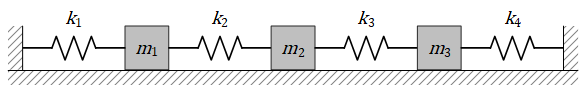
Fig. 63 Three masses connected by four springs on a frictionless surface
The case setup for this problem is very similar to the setup
for the tutorial 1D Wave Equation. You can define the
differential equations in spring_mass_ode.py and then define the
domain and the solver in spring_mass_solver.py.
The python scripts for this problem can be found at examples/ode_spring_mass/.
Defining the Equations
The equations of the system (142) can be coded using the sympy notation similar to tutorial 1D Wave Equation.
            from sympy import Symbol, Function, Number
from modulus.eq.pde import PDE


class SpringMass(PDE):
    name = "SpringMass"

    def __init__(self, k=(2, 1, 1, 2), m=(1, 1, 1)):

        self.k = k
        self.m = m

        k1 = k[0]
        k2 = k[1]
        k3 = k[2]
        k4 = k[3]
        m1 = m[0]
        m2 = m[1]
        m3 = m[2]

        t = Symbol("t")
        input_variables = {"t": t}

        x1 = Function("x1")(*input_variables)
        x2 = Function("x2")(*input_variables)
        x3 = Function("x3")(*input_variables)

        if type(k1) is str:
            k1 = Function(k1)(*input_variables)
        elif type(k1) in [float, int]:
            k1 = Number(k1)
        if type(k2) is str:
            k2 = Function(k2)(*input_variables)
        elif type(k2) in [float, int]:
            k2 = Number(k2)
        if type(k3) is str:
            k3 = Function(k3)(*input_variables)
        elif type(k3) in [float, int]:
            k3 = Number(k3)
        if type(k4) is str:
            k4 = Function(k4)(*input_variables)
        elif type(k4) in [float, int]:
            k4 = Number(k4)

        if type(m1) is str:
            m1 = Function(m1)(*input_variables)
        elif type(m1) in [float, int]:
            m1 = Number(m1)
        if type(m2) is str:
            m2 = Function(m2)(*input_variables)
        elif type(m2) in [float, int]:
            m2 = Number(m2)
        if type(m3) is str:
            m3 = Function(m3)(*input_variables)
        elif type(m3) in [float, int]:
            m3 = Number(m3)

        self.equations = {}
        self.equations["ode_x1"] = m1 * (x1.diff(t)).diff(t) + k1 * x1 - k2 * (x2 - x1)
        self.equations["ode_x2"] = (
            m2 * (x2.diff(t)).diff(t) + k2 * (x2 - x1) - k3 * (x3 - x2)
        )
        self.equations["ode_x3"] = m3 * (x3.diff(t)).diff(t) + k3 * (x3 - x2) + k4 * x3
Here, each parameter \((k's \text{ and } m's)\) is written as a function and is substituted as a number if it’s constant. This will allow you to parameterize any of this constants by passing them as a string.
Solving the ODEs: Creating Geometry, defining ICs and making the Neural Network Solver
Once you have the ODEs defined, you can easily form the constraints needed for optimization as seen in earlier tutorials.
This example, uses Point1D
geometry to create the point mass. You also have to define the time range of
the solution and create symbol for time (\(t\)) to define the
initial condition, etc. in the train domain. This code shows the
geometry definition for this problem. Note that this tutorial does not use the x-coordinate
(\(x\)) information of the point, it is only used to sample a
point in space. The point is assigned different values for variable
(\(t\)) only (initial conditions and ODEs over the time range). The code to
generate the nodes and relevant constraints is below:
            import numpy as np
from sympy import Symbol, Eq

import modulus
from modulus.hydra import instantiate_arch, ModulusConfig
from modulus.solver import Solver
from modulus.domain import Domain
from modulus.geometry.primitives_1d import Point1D
from modulus.domain.constraint import (
    PointwiseBoundaryConstraint,
    PointwiseBoundaryConstraint,
)
from modulus.domain.validator import PointwiseValidator
from modulus.key import Key
from modulus.node import Node

from spring_mass_ode import SpringMass


@modulus.main(config_path="conf", config_name="config")
def run(cfg: ModulusConfig) -> None:

    # make list of nodes to unroll graph on
    sm = SpringMass(k=(2, 1, 1, 2), m=(1, 1, 1))
    sm_net = instantiate_arch(
        input_keys=[Key("t")],
        output_keys=[Key("x1"), Key("x2"), Key("x3")],
        cfg=cfg.arch.fully_connected,
    )
    nodes = sm.make_nodes() + [
        sm_net.make_node(name="spring_mass_network")
    ]

    # add constraints to solver
    # make geometry
    geo = Point1D(0)
    t_max = 10.0
    t_symbol = Symbol("t")
    x = Symbol("x")
    time_range = {t_symbol: (0, t_max)}

    # make domain
    domain = Domain()

    # initial conditions
    IC = PointwiseBoundaryConstraint(
        nodes=nodes,
        geometry=geo,
        outvar={"x1": 1.0, "x2": 0, "x3": 0, "x1__t": 0, "x2__t": 0, "x3__t": 0},
        batch_size=cfg.batch_size.IC,
        lambda_weighting={
            "x1": 1.0,
            "x2": 1.0,
            "x3": 1.0,
            "x1__t": 1.0,
            "x2__t": 1.0,
            "x3__t": 1.0,
        },
        parameterization={t_symbol: 0},
    )
    domain.add_constraint(IC, name="IC")

    # solve over given time period
    interior = PointwiseBoundaryConstraint(
        nodes=nodes,
        geometry=geo,
        outvar={"ode_x1": 0.0, "ode_x2": 0.0, "ode_x3": 0.0},
        batch_size=cfg.batch_size.interior,
        parameterization=time_range,
    )
    domain.add_constraint(interior, "interior")
Next, you can define the validation data for this problem. The solution of this problem can be obtained analytically and the expression can be coded into dictionaries of numpy arrays for \(x_1, x_2, \text{and } x_3\). This part of the code is similar to the tutorial 1D Wave Equation.
            # add validation data
    deltaT = 0.001
    t = np.arange(0, t_max, deltaT)
    t = np.expand_dims(t, axis=-1)
    invar_numpy = {"t": t}
    outvar_numpy = {
        "x1": (1 / 6) * np.cos(t)
        + (1 / 2) * np.cos(np.sqrt(3) * t)
        + (1 / 3) * np.cos(2 * t),
        "x2": (2 / 6) * np.cos(t)
        + (0 / 2) * np.cos(np.sqrt(3) * t)
        - (1 / 3) * np.cos(2 * t),
        "x3": (1 / 6) * np.cos(t)
        - (1 / 2) * np.cos(np.sqrt(3) * t)
        + (1 / 3) * np.cos(2 * t),
    }
    validator = PointwiseValidator(
        nodes=nodes, invar=invar_numpy, true_outvar=outvar_numpy, batch_size=1024
    )
    domain.add_validator(validator)
Now that you have the definitions for the various constraints and domains complete, you can form the solver and run the problem. The code to do the same can be found below:
            # make solver
    slv = Solver(cfg, domain)

    # start solver
    slv.solve()
Once the python file is setup, you can solve the problem by executing the
solver script spring_mass_solver.py as seen in other tutorials.
The results for the Modulus simulation are compared against the
analytical validation data. You can see that the solution converges to
the analytical result very quickly. The plots can be created
using the .npz files that are created in the validator/ directory
in the network checkpoint.
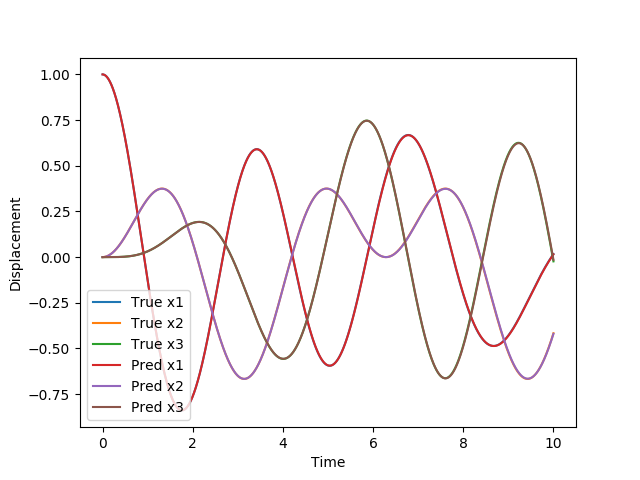
Fig. 64 Comparison of Modulus results with an analytical solution.