ImageFlip#
Overview#
ImageFlip performs coordinate transformation operations on single-channel grayscale images to achieve mirroring effects along the horizontal, vertical, or both axes. The operation preserves image content while changing pixel spatial relationships through address mapping transformations.
Three flip modes are supported:
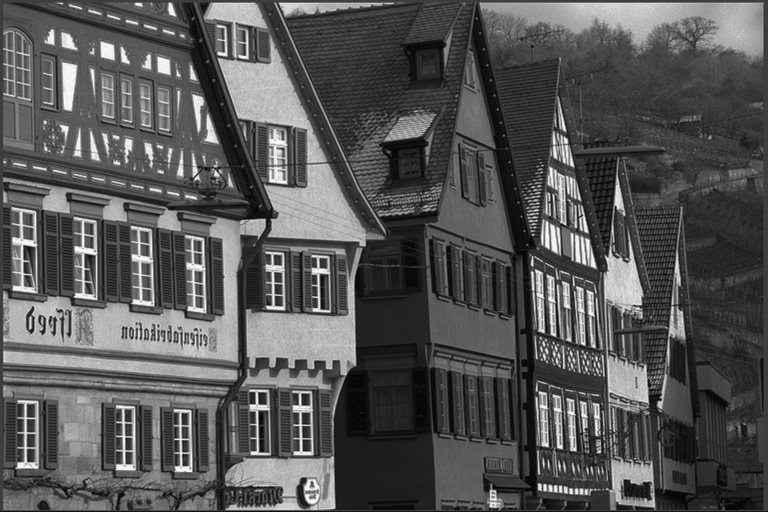
Horizontal Flip: Coordinate transformation along the vertical axis, reversing column ordering
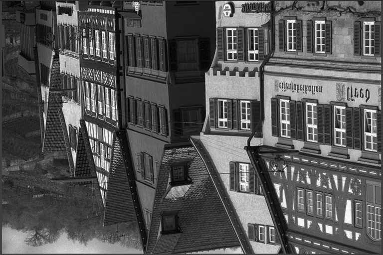
Vertical Flip: Coordinate transformation along the horizontal axis, reversing row ordering
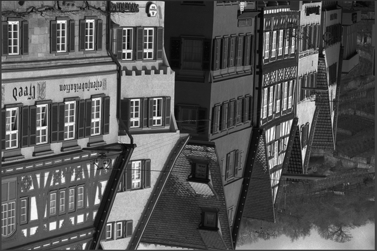
Combined Flip: Combined coordinate transformation reversing both row and column ordering
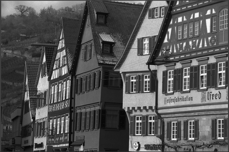
The following example demonstrates the effect of image flipping on a grayscale image:
Input Image |
Horizontal Flip |
|
|
Vertical Flip |
Combined Flip |
|
|
Algorithm Description#
The ImageFlip operator performs coordinate transformation operations using three different mathematical approaches:
Horizontal Flip:
Vertical Flip:
Combined Flip:
Where:
\(\text{dst}(x, y)\) is the pixel value at coordinates (x, y) in the output image
\(\text{src}(x, y)\) is the pixel value at coordinates (x, y) in the input image
\(W\) is the image width
\(H\) is the image height
Parameters#
Input/Output image type: 8-bit unsigned single-channel grayscale
Flip Direction: Runtime selectable (horizontal, vertical, combined)
Implementation#
The implementation uses tile-based processing of the input image, where each Tile(i,j) denotes tile coordinates: i = horizontal tile number, j = vertical tile number.
RDF configurations use tile dimensions of \(256 \times 128\) pixels for optimal performance and employ double buffering to overlap computation and data transfer.
Horizontal Flip:
- Input RDF: Reads Tile(i,j)
Handle: srcHdl
Tile buffer: input_v in VMEM
Dimensions: (\(TW \times TH\))
Configuration:
.scanOrder(HORIZONTAL_REVERSED)for tile column reversal
- VPU Processing: Horizontal pixel transformation
t(x,y) = t(tw-x-1,y) Vector operations: 32-wide parallel processing
Vector Permute Instruction (
vpermute): Performs efficient pixel reordering within vector registers for horizontal flipping using a reverse indexed pattern.Reverse address generation for pixel column reversal
- VPU Processing: Horizontal pixel transformation
- Output RDF: Writes Tile(i,j) to Tile(w-i-1,j)
Handle: dstHdl
Tile buffer: output_v in VMEM
Dimensions: (\(TW \times TH\))
Vertical Flip:
- Input RDF: Reads Tile(i,j)
Handle: srcHdl1
Tile buffer: input_v in VMEM
Dimensions: (\(TW \times TH\))
Configuration:
.scanOrder(VERTICAL_REVERSED)for tile row reversal
- VPU Processing: Vertical pixel transformation
t(x,y) = t(x,th-y-1) Vector operations: 32-wide parallel processing
Reverse address generation for pixel row reversal
- VPU Processing: Vertical pixel transformation
- Output RDF: Writes Tile(i,j) to Tile(i,h-j-1)
Handle: dstHdl1
Tile buffer: output_v in VMEM
Dimensions: (\(TW \times TH\))
Combined Flip:
- Input RDF: Reads Tile(i,j)
Handle: srcHdl2
Tile buffer: input_v in VMEM
Dimensions: (\(TW \times TH\))
Configuration:
.scanOrder(HORIZONTAL_REVERSED | VERTICAL_REVERSED)for dual tile reversal
- VPU Processing: Combined pixel transformation
t(x,y) = t(tw-x-1,th-y-1) Vector operations: 32-wide parallel processing
Vector Permute Instruction (
vpermute): Performs efficient pixel reordering within vector registers for horizontal flipping using a reverse indexed patternCompound address generation for dual pixel transformation
- VPU Processing: Combined pixel transformation
- Output RDF: Writes Tile(i,j) to Tile(w-i-1,h-j-1)
Handle: dstHdl2
Tile buffer: output_v in VMEM
Dimensions: (\(TW \times TH\))
Performance#
Execution Time is the average time required to execute the operator on a single VPU core.
Note that each PVA contains two VPU cores, which can operate in parallel to process two streams simultaneously, or reduce execution time by approximately half by splitting the workload between the two cores.
Total Power represents the average total power consumed by the module when the operator is executed concurrently on both VPU cores.
Idle power is approximately 7W when the PVA is not processing data.
For detailed information on interpreting the performance table below and understanding the benchmarking setup, see Performance Benchmark.
ImageSize |
Format |
Direction |
Execution Time |
Submit Latency |
Total Power |
|---|---|---|---|---|---|
256x128 |
U8 |
HORIZONTAL |
0.016ms |
0.019ms |
10.336W |
1280x720 |
U8 |
HORIZONTAL |
0.077ms |
0.024ms |
14.858W |
1920x1080 |
U8 |
HORIZONTAL |
0.153ms |
0.029ms |
15.459W |
3840x2160 |
U8 |
HORIZONTAL |
0.576ms |
0.030ms |
15.158W |
1920x1080 |
U8 |
VERTICAL |
0.153ms |
0.030ms |
15.06W |
1920x1080 |
U8 |
BOTH |
0.153ms |
0.030ms |
15.462W |
1920x1080 |
Y8 |
HORIZONTAL |
0.153ms |
0.029ms |
15.459W |
1920x1080 |
Y8 |
VERTICAL |
0.153ms |
0.030ms |
15.06W |
1920x1080 |
Y8 |
BOTH |
0.153ms |
0.031ms |
15.459W |
1920x1080 |
Y8_ER |
HORIZONTAL |
0.153ms |
0.030ms |
15.459W |
1920x1080 |
Y8_ER |
VERTICAL |
0.153ms |
0.030ms |
15.06W |
1920x1080 |
Y8_ER |
BOTH |
0.153ms |
0.031ms |
15.459W |