FASTCornerDetector

Overview

The Features from Accelerated Segment Test (FAST) algorithm is a widely used method for detecting corners. Its main advantage is low computational complexity. The algorithm’s details can be found in [1], [2], and [3].

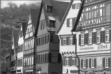
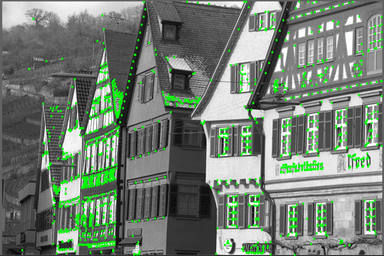
One of the main disadvantages of the FAST corner detector is multiple detections of corners in proximity; therefore, Non-Maximum Suppression (NMS) is often used to refine the output. Since the original algorithm only classifies pixels into corners and non-corners and does not compute a corner response function, NMS cannot be directly applied to the resulting corners. The current implementation follows OpenCV’s approach, which calculates the maximum threshold that makes the target pixel a FAST corner and uses this threshold (called the score) as the input for NMS. More details can be found in [4]. Other methods to calculate scores, such as computing the sum of absolute differences between surrounding pixels and center pixels, are also available in the literature. The sample input image and output results are shown in the following figures, where the green dots are the detected corners.

Figure 1: Sample input image (left) and output results (right). Data type is uint16_t, threshold is 15428 and NMS is ON.

Design Requirements

1. Data type supports uint8_t, uint16_t, int8_t and int16_t.

2. Supports a circle radius of 3 and an arc length of 9.

3. NMS can be ON or OFF.

4. The output location is X-Y interleaved float. Note that the order of locations is implementation-specific; additional sorting may be needed to compare locations from different implementations.

5. The image border extension type can be constant or replicate.

6. TopK feature selection is controlled by the numTopKFeatures parameter. When set to 0 (default), all detected corners are returned. When set to a value in [1, PVA_FAST_CORNER_MAX_TOPK_FEATURES (250000)], the operator returns approximately the K highest-scoring corners using histogram-based score thresholding.

Implementation Details

Quick Rejection

To further reduce computational complexity, a quick rejection method is adopted. This method conducts an initial test to eliminate pixels that are not corners, allowing only non-rejected pixels to undergo further testing and score calculation if they are corners. The quick rejection method described in “High-speed test” of [2] refers to a configuration with a circle radius of 3 and an arc length of 12.

The proposed scheme tests pixel P1, P5, P9, and P13 (shown in the following figure), which are located at 90-degree intervals on the circle. The implementation computes the minimum and maximum of these four test pixels. If the minimum is at least \(I_{p}-t\) and the maximum is at most \(I_{p}+t\) (where \(I_{p}\) is the central pixel’s intensity and \(t\) is the threshold), all four test pixels are close to the center, and the pixel is rejected as a non-corner.

The correctness of this approach relies on the following observation: for a pixel to be a FAST corner with arc length 9, it needs at least one contiguous arc of 9 pixels that are all brighter (or all darker) than the center by at least \(t\). If even the most extreme of the four cardinal test pixels (i.e., the minimum or maximum) is within the threshold range, then the second-most-extreme pixel is guaranteed to be within range as well, meaning no contiguous arc of 9 brighter or darker pixels can exist. Therefore, if the overall minimum and maximum of the four test pixels are both within the threshold range, at least one arc criterion fails and the pixel cannot be a corner.

This min/max approach is computed efficiently using simultaneous sort instructions (dvsort2), requiring approximately 7 SIMD instructions compared to approximately 30 instructions for individually checking each test pixel position. As the current implementation uses SIMD instructions to process 1x32 pixels as a chunk, it is also necessary to test a contiguous block of 1x32 pixels and reject them as a whole if all satisfy the rejection criteria. In other words, if there is even one pixel that does not meet the rejection criteria, this 1x32 pixel chunk will not be rejected.

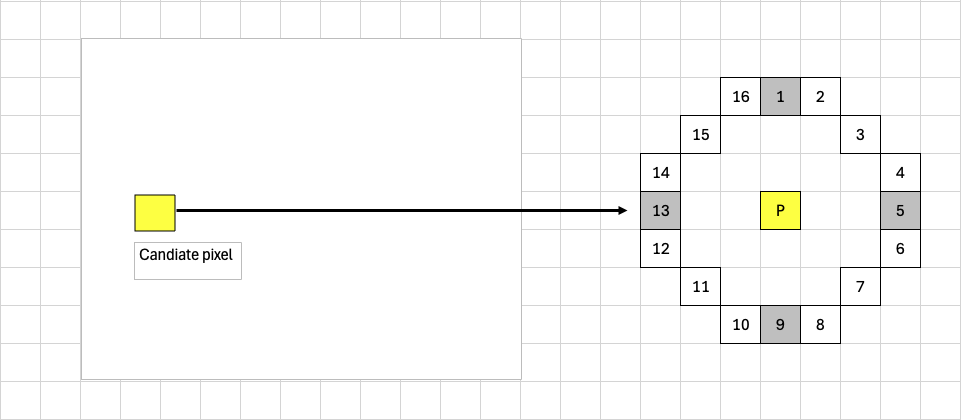
Figure 2: Quick Rejection Illustration

The rationale behind quick rejection is that corners are quite sparse in practical scenarios, e.g., less than 1% of the image’s total pixels. The time consumption after adopting quick rejection becomes quick_rejection_time + non_rejection_ratio * score_calculation_time, leading to two implications:

1. If quick_rejection_time is smaller than score_calculation_time, overall time consumption will be reduced using quick rejection when non_rejection_ratio is small.

2. In rare cases where non_rejection_ratio is relatively large (e.g., 10%), overall time consumption may increase compared to not using quick rejection.

TopK Feature Selection

When TopK is enabled (numTopKFeatures > 0), the operator returns approximately the numTopKFeatures highest-scoring corners rather than all detected corners. This is achieved using a two-pass histogram-based approach executed entirely on the VPU:

Packing pass: During the normal score computation and packing stage, all detected corners (up to an intermediate capacity of 250,000) are packed into DRAM along with their scores via SQDF. Simultaneously, a 256-bin histogram of corner scores is accumulated in VMEM using vectorized histogram instructions. Periodic reductions transfer the vector histogram lanes into a scalar histogram to prevent overflow.

Threshold computation: After all tiles are processed, the scalar histogram is scanned from the highest bin downward to find the score threshold at which approximately numTopKFeatures corners have scores at or above that threshold. The lookahead logic ensures the threshold is set conservatively so that the number of features passing the filter does not significantly exceed numTopKFeatures.

Filtering pass: The packed corners are read back from DRAM in batches via SQDF. Each batch is filtered on the VPU: only corners whose score meets or exceeds the computed threshold are retained. The surviving corners are converted to float X-Y format and written to the output buffer.

For uint8_t and int8_t data types, each histogram bin corresponds to a single score value (bins 0–255). For uint16_t and int16_t data types, scores are mapped to bins via right-shift by 8 (i.e., bin = score >> 8), so each bin covers 256 score values. This results in coarser threshold granularity for 16-bit types.

When TopK is disabled (the default), behavior is unchanged from previous releases.

Dataflow Configuration

1. Use RDF dataflow to transfer tiles from DRAM to VMEM, similar to a 7x7 2D filtering process. For each tile, calculate scores and transfer them back from VMEM to DRAM as a height * width image in tight layout, with values representing scores. This step prepares for overlapping tiles required by NMS.

2. Use RDF dataflow again to transfer the score-valued image from DRAM to VMEM, akin to a 3x3 2D filtering operation. For each tile, perform NMS; for each non-zero NMS output, calculate its location within the entire image and output it in X-Y interleaved format. SQDF dataflow transfers these locations from VMEM to DRAM. The number of locations varies among tiles, necessitating a similar mechanism to maintain related states on both device and host sides. More information can be found in the documentation regarding the MinMaxLoc operator’s output.

When NMS is OFF, the above two steps can be merged into one step. In this case, the scores do not need to be transferred back to DRAM, as the locations can be directly calculated based on the scores. The host code uses flags to set up different dataflows. The device code uses separately built binaries for NMS being either ON or OFF to avoid branches in the device code.

When TopK is enabled, additional SQDF dataflows are configured for transferring packed corner locations and scores between VMEM and DRAM. Two intermediate DRAM buffers are allocated at operator creation time: one for packed locations (uint32_t, up to 250,000 entries) and one for packed scores (uint16_t, up to 250,000 entries), totaling approximately 1.5 MB. The TopK filtering pass reuses the existing location SQDF for writing the final filtered output.

Different Data Types Support

The support for different data types has several implications:

1. From the algorithm’s perspective, the score result is always larger than or equal to 0 since the current corner response function uses the absolute difference between the central pixel and the surrounding pixels. Although the final output is float type, the intermediate representation always uses int16_t type. This is independent of the data type of the score, since otherwise uint8_t type can only support a maximum coordinate value of 255.

2. From the VPU implementation’s perspective, the PVA hardware constraint requires that double vector load/store must be 2-byte-aligned. Therefore, two single byte-type vector load instructions must be used to populate a double vector of byte type if an address is 1-byte-aligned.

3. From the performance perspective, when comparing the implementation of signed and unsigned types, the device code only differs in the variants of the load and store instructions used (e.g., vuchar_load versus vchar_load), which has no performance impact. Additionally, the support for different data types has been separately built into different device code binaries to avoid branch penalties. Combined with NMS and TopK options, this results in a total of 16 different device code binaries (4 data types × 2 NMS options × 2 TopK options).

Performance

Execution Time is the average time required to execute the operator on a single VPU core. Note that each PVA contains two VPU cores, which can operate in parallel to process two streams simultaneously, or reduce execution time by approximately half by splitting the workload between the two cores.

Total Power represents the average total power consumed by the module when the operator is executed concurrently on both VPU cores. Idle power is approximately 7W when the PVA is not processing data.

For detailed information on interpreting the performance table below and understanding the benchmarking setup, see Performance Benchmark.

ImageSize	DataType	NMS	TopK	TestData	Corner Count	Execution Time	Submit Latency	Total Power
1024x1024	U8	inf	inf	Random	N/A	1.687ms	0.029ms	NoneW
1920x1080	U8	inf	inf	Random	N/A	3.334ms	0.029ms	NoneW
1920x1080	U8	inf	inf	kodim08_grayscale_1920x1080_u16	N/A	1.801ms	0.026ms	NoneW
1024x1024	U16	inf	inf	Random	N/A	2.891ms	0.029ms	NoneW
1920x1080	U16	inf	inf	Random	N/A	5.704ms	0.032ms	NoneW
1920x1080	U16	inf	inf	kodim08_grayscale_1920x1080_u16	N/A	3.609ms	0.029ms	NoneW

Note: For performance measurements using real images, the uint8_t data type case uses the same source image as the uint16_t case. During image loading, the data is converted from uint16_t to uint8_t on the fly, ensuring both cases operate on identical image content.

Reference

1. https://docs.opencv.org/4.x/df/d0c/tutorial_py_fast.html

2. https://en.wikipedia.org/wiki/Features_from_accelerated_segment_test

3. https://docs.nvidia.com/vpi/algo_fast_corners_detector.html#algo_fast_corners_detector_overview

4. https://stackoverflow.com/questions/67306891/algorithm-behind-score-calculation-in-fast-corner-detector