Shader Profiler#
GPU Trace includes a Shader Profiler tool for analyzing the performance of SM-limited workloads. It helps you, as a developer, identify the reasons that your shader is stalling and thus lowering performance. With the data that the shader profiler provides, you can investigate, at both a high- and low-level, how to get more performance out of your shaders. The Shader Profiler supports D3D12 and Vulkan profiling of HLSL, GLSL, and Slang shaders.
The Shader Profiler can be accessed in the bottom section of a GPU Trace report that was collected with “Real-Time Shader Profiling” enabled. A source view is also available as a secondary tab to the GPU Trace timeline.
Sections#
The Shader Profiler has the following tabbed sections:
Shaders Pipelines: this section provides a hierarchical breakdown of the shaders executed in the selected time range. It is the primary jumping-off point for understanding how your shaders performed.
Flame Graph: this section provides a visualization of the execution of the high-level functions (HLSL / GLSL / Slang) and their called sub-functions.
Top-Down / Bottom-Up: these sections provide a hierarchical breakdown of the high-level functions (HLSL / GLSL / Slang) and their called sub-functions.
Hotspots: this section reports the source-lines for which the Top Stalls are discovered.
RT Live State: this section reports the ray tracing live state information for ray tracing applications.
Instruction Mix: this section provides a breakdown of the instruction types, input dependencies and output stall locations in your shader(s). When the Source View is visible, this view is contextual to the currently selected source line(s).
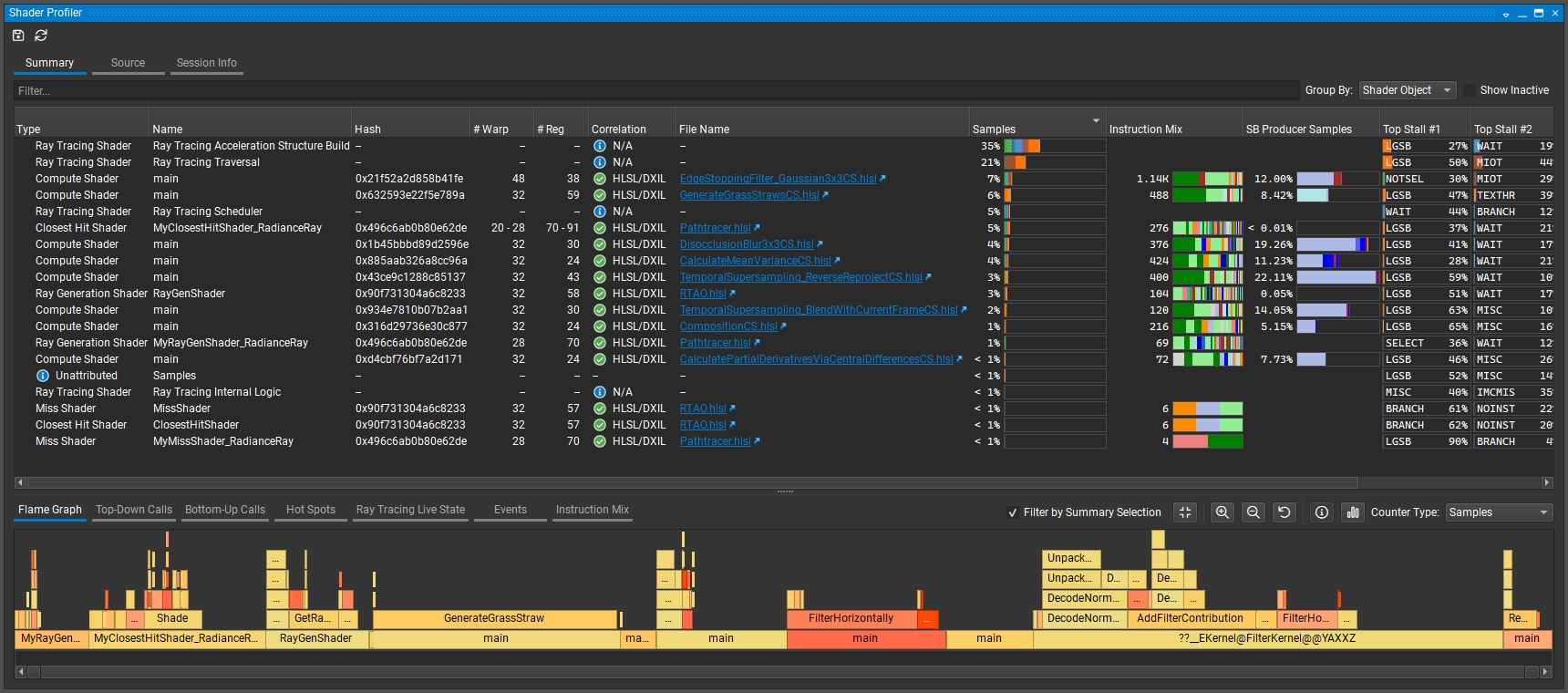
Shader Pipelines#
This section provides a hierarchical breakdown of the shaders used by the range that was profiled. It is the primary jumping-off point for understanding how your shaders performed.
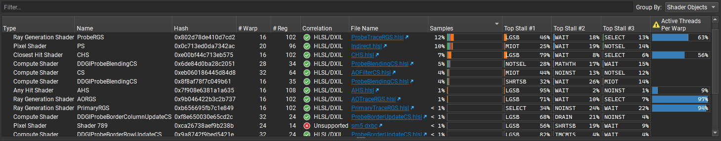
This section presents a table of all of the shaders within a range alongside how each performed. At the root, there is a ‘Session’ element that represents all samples for the entire range. Below it, the shaders are grouped depending on the Group By setting of the view. Grouping by Shader flattens the tree; grouping by Pipeline hierarchically lays out all samples according to the pipeline to which they belong.
The left-hand side of the information panel presents information by which you can classify each shader.
Type: indicates the kind of hierarchy for elements below.
Name: the name of the shader / pipeline for which results were collected.
Hash: displays a unique hash of application level shader information (e.g., bytecode).
# Warp: indicates the maximum theoretical warp occupancy. At the shader instance level, this is the maximum number of warps that can fit concurrently in an SM, if this shader was run in isolation. At the pipeline level, it shows the range of values across all shader stages’ shader instances. Hover over this cell for a tooltip that reports which resource(s) limited the theoretical warp occupancy. When dynamic conditions (such as the # of primitives) affect the calculation, a range of values is displayed for the two extreme cases.
# Reg: indicates the registers per thread needed by a shader.
Smem: indicates the bytes of attributes needed by a 3D shader per warp, or the shared memory allocated for a compute shader per thread group.
CTA Dim: indicates the thread group size used by a shader (i.e., HLSL numthreads, GLSL local_size, Hull / Tessellation Control patch_size).
Correlation: reports the success or failure of reading debug and correlation information for the shader that was profiled. Hover over this cell for a tooltip that reports detailed information about the operation, including the files in which debug information was read.
File Name: the file from which this shader was generated.
The center-right side presents the performance of the row in question, including the top stalls for each row and all stall reasons.
See Stall Reasons for a full listing and description of stall reasons.
When sampling, some samples may be reported as Unattributed. Samples in this row either failed correlation, or represent internal operation of the GPU that this sampler does not report. These samples can generally be ignored, except in the case where the results are of a high quantity, in which case we recommend you save this report to communicate this issue to the Nsight Graphics team.
Samples: reports the total summation of samples collected for this row.
Top Stall #1: reports the stall reason with the highest incidence for the row in question.
Top Stall #2: reports the stall reason with the 2nd highest incidence for the row in question.
Top Stall #3: reports the stall reason with the 3rd highest incidence for the row in question.
The rightmost side presents the execution counters of the row in question, including instruction executed counts, thread-instruction executed counts and thread divergence.
Instructions Executed: reports number of instructions executed.
Thread Instructions Executed: reports sum of instructions executed of all threads (this is up to 32 * “Instruction Executed” as each warp has 32 threads).
Thread Instructions Executed Pred On: same as “Thread Instructions Executed” but only count the predicated-on threads (the predicated-on threads execute the current instruction while the predicated-off threads skip it).
Active Threads Per Warp: reports thread divergence that the average predicated-on threads are executed per instruction.
Active Threads Per Warp = Thread Instructions Executed Pred On / (Instructions Executed * 32)
Note
By default some columns are hidden. The visibility of columns can be toggled by right-clicking on the table’s header.
Flame Graph#
This section provides a visualization of software execution. This is based on function calls while the root functions are displayed as aligned color bars at the bottom and the called functions are recursively stacked above them. It is only available when the input shader bytecode has debug information (e.g., adding “/Zi” option for dxc compiling DXIL bytecode).
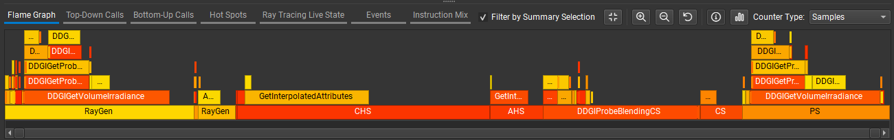
Every color bar represents a function. The width of the bar is proportional to the number of samples / execution counters.
The y-axis shows the function call depth, ordered from root at the bottom to leaf at the top.
The x-axis shows the size of samples / execution counters, across different shaders.
Interact with Source, Top-Down Calls and Bottom-Up Calls by clicking a color bar or the Go To… actions in the context menu.
Focus on one function and show callers and callees by clicking action Show Butterfly View in the context menu.
Focus on one function and aggregate samples from every instance into a single root node, by clicking Aggregate Across all Calls in the context menu.
Top-Down Calls#
This section provides a hierarchical breakdown of the high-level (HLSL / GLSL / Slang) functions and their called sub-functions. It is only available when the input shader bytecode has debug information (e.g., adding “/Zi” option for dxc compiling DXIL bytecode). Samples / execution counters are aggregated to the function level. Links can be clicked to navigate to the source line of function definition or where a function is called within the Source section.
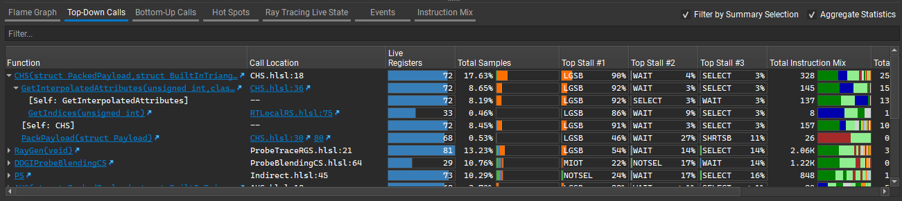
Function: the name of the function. Expand to see other functions that called by it.
Call Location: the file and line that this function is called.
Bottom-Up Calls#
Similar to Top-Down Calls, this section provides a hierarchical breakdown of the high-level (HLSL / GLSL / Slang) functions and their caller functions. This is only available when the input shader bytecode has debug information (e.g., adding “/Zi” option for dxc compiling DXIL bytecode). Samples / execution counters are aggregated to the function level. Links can be clicked to navigate to the source line of function definition or where a function is called within the Source section.
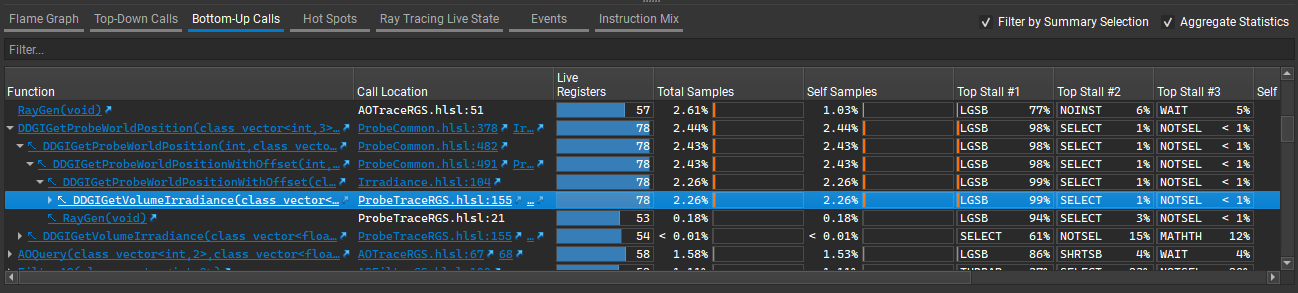
Function: the name of the function. Expand to see in what functions it is called, and to find out the weights of samples / execution counters from different caller functions.
Call Location: the file and line that this function is called.
Hot Spots#
This section reports the source-lines for which the Top Stalls are discovered. Lines within this table can be double-clicked to navigate to the source line in question within the Source section. The display can also be toggled between High-Level and Intermediate/Lower level by changing the Type selection.
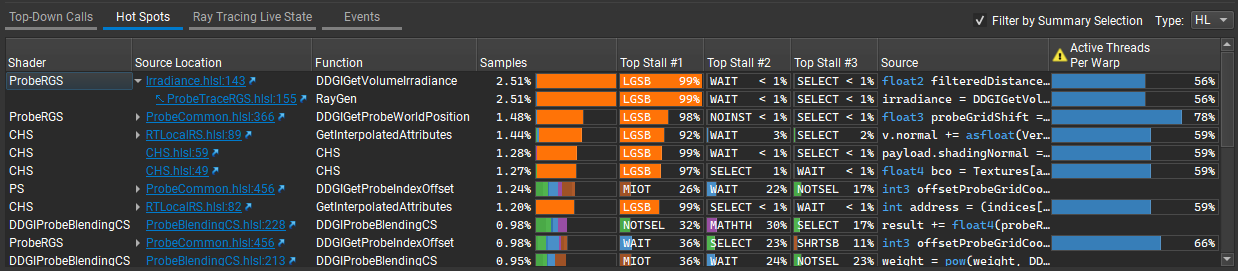
Shader: the shader to which this line belongs.
Source Location: the file and line of this hot spot. Expand to see the call path.
Function: the name of the function to which this hot spot belongs.
Source: the source for the particular hot spot.
Ray Tracing Live State#
This section reports the ray tracing live state information for ray tracing applications. Source/IL location links within this table can be clicked to navigate to the source/IL line in question within the Source section.
Variables initialized before an (HLSL) TraceRay or (GLSL) traceRayEXT call, and used after it, are Live State that need to be maintained across the call while invoking hit and miss shaders. For improved performance, we recommend trying to minimize the amount of live state.
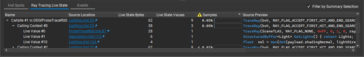
Name: shows the callsite / calling context / live value names (identifiers).
Source Location: reports the source location from which this live state information comes.
Live State Bytes: reports the size of this live state information.
Live State Values: reports the number of live values reloaded / defined at the particular location.
Samples: reports the cost of the trace ray call in question, including live state loads, but it does not include the latency penalty on the consumer of the live state loads.
Source Preview: shows the source preview for the particular live state inforamtion.
IL Preview: shows the IL preview for the particular live state information.
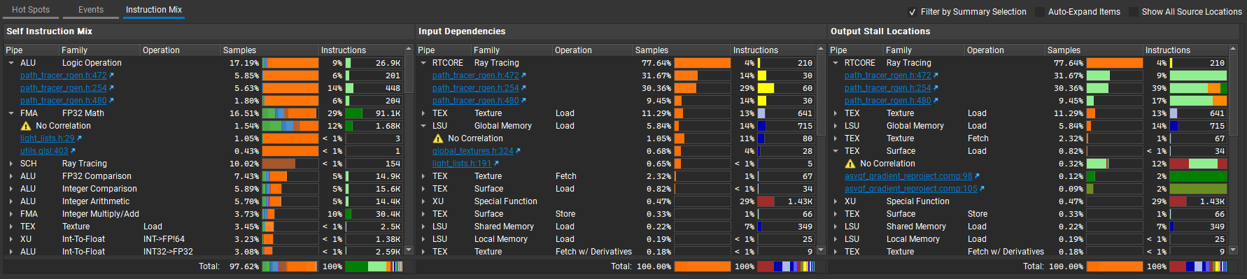
Instruction Mix#
The Instruction Mix view provides a breakdown of the instruction types, input dependencies and output stall locations in your shader(s). It is context-sensitive to the selection in the Shaders and Source views.
The Instruction Mix view is useful for navigating through instruction level dependencies. Variable latency instructions — such as memory accesses, transcendental math functions, and warp level primitives — are called scoreboard producers. Instructions that use the results of scoreboard producers, or that reuse the registers from scoreboard producers, are called scoreboard consumers. Stall reasons such as “long scoreboard” appear on the scoreboard consumer instructions, but are actually caused by the corresponding scoreboard producers instructions.
The section contains three tables:
Self Instruction Mix: this table provides a breakdown of instruction types and number of samples attributed to each instruction type within the current selection. Each sub-item contains a hyperlink that can be clicked to jump to that location in the Source View.
Input Dependencies: this table provides a list of scoreboard producer instruction categories that the current selection is dependent upon. Each sub-item contains a hyperlink that can be clicked to jump to the location of the scoreboard producer in the Source View.
Output Stall Locations: this table provides a list of scoreboard producer instruction categories within the current selection. Each sub-item contains a hyperlink that can be clicked to jump to the consumer of the given scoreboard in the Source View.
Each table has the same columns available:
Pipe: hardware pipe used to process the instruction.
Family: type of work that the instruction performs.
Operation: type of operation of the given work type that the instruction performs.
Samples: number of samples attributed to the instruction category or location.
Instructions: number of instructions or instruction mix corresponding to the given category or location.
The view provides controls to adjust how data is displayed:
Filter by Summary Selection: if checked, results reflect the current selected item(s) on the Shaders view; otherwise the selection is ignored and results for all shaders are shown. This does not impact data shown while in the Source view.
Auto-Expand Items: if checked, all top-level cells automatically expand to reveal sub-items with hyperlinks.
Show All Source Locations: if checked, all source locations are listed as sub-items under each top-level cell; otherwise only the top 3 locations by number of samples are shown.
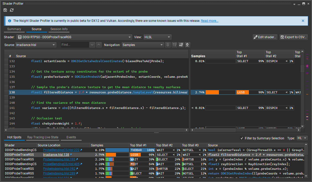
Source Tab#
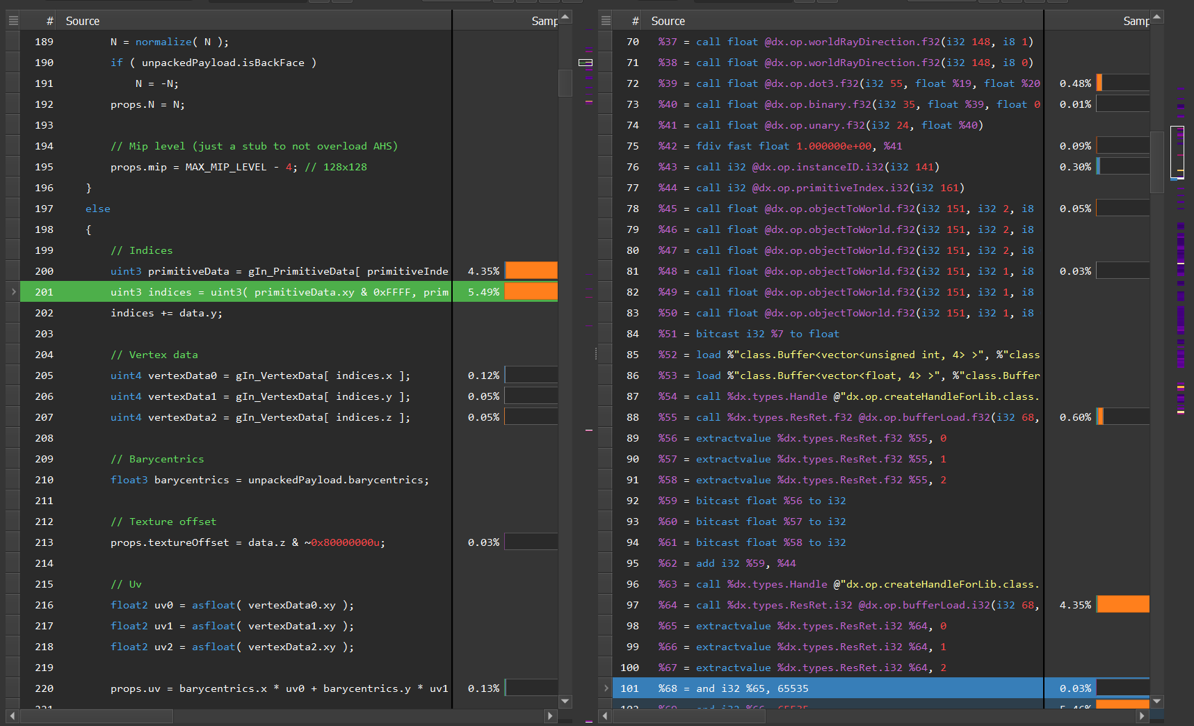
This section reports a per-line breakdown of the performance of your shaders. It includes several visualization modes, including high-level source reports, side-by-side high-level source to lower-level correlation, and interleaved high-level source within lower-level source through a mixed mode view.
There are a few top-level controls that control which shader is viewed and how that shader is viewed.
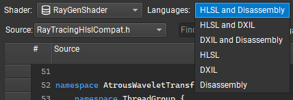
Shader: select the shader that you would like to view.
Languages: change the source display to show high-level language, a lower-level language, or alternatively, high-level language alongside a lower-level language.
Source: because shaders can be compiled from a main file and several includes, this selector allows you to select which particular source file you wish to investigate.
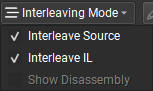
Interleaving Mode: controls how higher-lever source is interleaved within the view (only available for lower-level source views).
Once a shader and view is selected, you can use one of several navigation tools to navigate within the shader source.

Find: enter a text string to find. This is useful for finding variables, methods, or register names.
 : navigate to the row with the highest value in the corresponding stall reason column.
 : navigate to the row with the next higher value in the corresponding stall reason column.
 : navigate to the row with the next lower value in the corresponding stall reason column.
 : navigate to the row with the lowest value in the corresponding stall reason column.
For many uses cases, you likely want to start by navigating to the highest value, and from there navigate progressively high values until you have planned your next action.
In addition to using the navigation buttons above, you may use the scrollbar with embedded heatmap to identify areas within the source file that are of interest given a high sample count.
To copy lines, select the lines in question and use the system shortcut to copy to the clipboard. Multiple successive lines can be selected with Shift+click; individual lines can be selected with Ctrl+click.
Source Navigation
Go Backward / Forward: navigate to the previous or next positions in the source file.

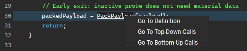
Go To Definition: navigate to the definition of a function from where the function is called. The function call is displayed as a hyperlink.
Go To Top-Down / Bottom-Up Calls: right-click the hyperlink and you are able to go to the corresponding item in Top-Down Calls or Bottom-Up Calls.
Shader Profiling for SM Limited Workloads#
The Shader Profiler is a tool for analyzing the performance of SM-limited workloads. It helps you, as a developer, identify the reasons that your shader is stalling and thus lowering performance. With the data that the Shader Profiler provides, you can investigate, at both a high- and low-level, how to get more performance out of your shaders. The Shader Profiler currently supports D3D12 and Vulkan APIs.
How do I use it?#
The Shader Profiler is available when collecting a GPU Trace with Real-Time Shader Profiling enabled. On some architectures, Real-Time Shader Profiling is only supported with specific metric sets, this is indicated by a “flame” icon next to the metric set name.
Key Concepts#
The shader profiler should be used to optimize latency-bound shaders. These types of shaders often have signatures of these forms:
SM Activity and SM Occupancy are high. (If not, improve these first.)
SM Throughput is low.
Cache Throughputs (L1TEX, L1.5, L2) are low or middling.
If SM Throughput is high, the shader is likely computationally-bound, and better solved through a GPU Trace workflow.
Average Warp Latency#
The average warp latency is the number of cycles that an average warp was resident on the GPU. The Samples% indicates the percent of the average warp latency occupied by a given shader, function, or PC. Sorting by Samples reveals the regions of code with the highest contribution to latency. After identify top latency contributors, determine next steps by inspecting stall reasons.
Interpreting Sample Locations#
Stalls are reported at the PC where a warp was unable to make progress. In many cases, this is due to an execution or data dependency on a prior instruction. For example, the following code may report a large number of samples on the line of code that consumes texResult, but the real culprit is the data producer g_MeshTexture.Sample().
float4 texResult = g_MeshTexture.Sample(MeshTextureSampler, In.TextureUV);
Output.RGBColor = texResult * In.Diffuse;
Note that samples can appear in the shadow of a taken branch — that is, on the instruction following a branch, even if that instruction is not executed — because the branch is still resolving at the time of the sampling.
if (constantBuffer.ConditionWeExpectToBeFalse)
{
     texResult = ...; // samples in the shadow of a branch
     output = dot(color, textResult);
}
else
{
     output = dot(color, constant);    // expect all samples to fall here
}
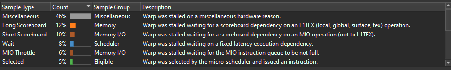
Stall Reasons#
Stall reasons explain why a warp was unable to issue an instruction. Each stall reason is provoked by a distinct set of conditions or instructions; by eliminating those conditions or transforming code from one set of instructions to another, you can reduce stalls.
Barrier: Compute warps are waiting for sibling warps at a GroupSync.
If the thread group size is 512 threads or greater, consider splitting it into smaller groups. This can increase eligible warps without affecting occupancy, unless shared memory becomes a new occupancy limiter.
Review whether all GroupSyncs are really necessary.
Dispatch Stall: A pipeline interlock prevented instruction dispatch for a selected warp.
If dispatch stalls are higher than 5%, please file a bug with NVIDIA.
Drain : Exited warp is waiting to drain memory writes and pixel export.
LG Throttle: Input FIFO to the LSU pipe for local and global memory instructions is full.
Avoid using thread-local memory.
Are dynamically indexed arrays declared in local scope?
Does the shader have excess register pressure causing spills?
Eliminate redundant global memory accesses (UAV accesses).
Data organization: pack UAV or SRV data to allow 64-bit or 128-bit accesses in place of multiple 32-bit accesses.
Long Scoreboard: Waiting on data dependency for local, global, texture, or surface load.
Find the instruction or line of code that produces the data being waited upon; that instruction is the culprit.
Consider transforming a lookup table into a calculation.
Consider transforming global reads in which all threads read the same address into constant buffer reads.
If L1 hit rate is low, try to improve spatial locality (coalesced accesses).
If VRAM Throughput is high, try to improve spatial locality (coalesced accesses).
Math Pipe Throttle: A math pipe input FIFO is full (FMA, ALU, FP16+Tensor).
This stall reason implies being computationally bound. Use GPU Trace to best determine how to move computation to a different execution unit.
Membar : Waiting for a memory barrier to return.
Memory barriers are issued by GroupMemoryBarrier, DeviceMemoryBarrier, AllMemoryBarrier, and their GroupSync variants.
Review whether the specified scope of each barrier in the shader is really needed. Group-level barriers resolve much faster than Device-level.
Review whether a memory barrier is needed at all. A compute shader where each thread writes to a unique UAV location does not require a memory barrier.
MIO Throttle: The input FIFO to MIO is full.
May be triggered by local, global, shared, attribute, IPA, indexed constant loads (LDC), and decoupled math.
Misc: A stall reason not covered elsewhere.
Not Selected: Warp was eligible but not selected, because another warp was.
High “not selected” could indicate an opportunity to increase register or shared memory usage (lowering occupancy) without impacting performance. This opens the doors to greater shader complexity or improved quality.
Selected: Warp issued an instruction. Technically not a stall.
Short Scoreboard: Waiting for short latency MIO or RTCORE data dependency.
TEX Throttle: The TEXIN input FIFO is full.
Try issuing fewer texture fetches, surface loads, surface stores, or decoupled math operations.
Check whether the shader is using decoupled math (usually to be avoided).
Consider converting texture lookups or surface loads into global memory lookups (UAVs). Texture can accept 4 threads’ requests per cycle, whereas global accepts 32 threads.
Wait: Waiting for coupled math data dependency (FMA, ALU, FP16+Tensor).
Hot Spots#
Hot spots identify the top locations that have the most hit samples. This listing presents an actionable way of identifying and jumping to high-impact areas of the given report.
Ray Tracing Live State#
Ray Tracing Live State lists ray tracing live state information for ray tracing applications and presents an actionable way of identifying and jumping to high-impact areas of the given report.
Variables initialized before an (HLSL) TraceRay or (GLSL) traceRayEXT call, and used after it, are Live State that need to be maintained across the call while invoking hit and miss shaders. For improved performance, we recommend trying to minimize the amount of live state.
Source Correlation#
The Shader Profiler has the ability to correlate the samples that are gathered to source-level lines. This allows you, as the user, to determine, on a line-by-line basis, how your code is running. There are two types of correlation that are supported: high-level shader language correlation and GPU shader assembly microcode correlation. High-level shader language correlation prepares a listing of your shaders source code, and alongside it, a chart of the samples that landed on each particular line. High-level correlation is effective at grounding you to the code you are most familiar with, which is the shader source itself. For users who have access to the Pro builds of Nsight Graphics, and who wish to dive into the lower-level shader assembly, a disassembly view is provided for individual instruction association of samples. For non-Pro users, the disassembly view still shows instruction-range correlation. Low-level source correlation views allow interleaving of higher-level source code. This can be configured through the Interleaving Mode dropdown menu.