Behavior Analytics

Overview

Introduction

The Behavior Analytics microservice is implemented in Python and leverages the Python Multiprocessing library for parallel processing.

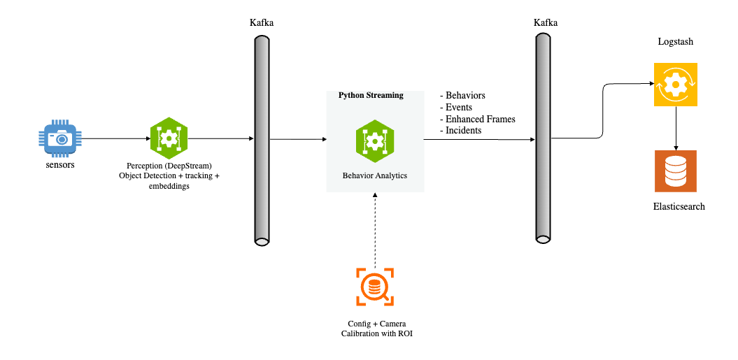
The perception layer processes camera or video input streams, performing sequential frame analysis for object detection and tracking. It generates object embeddings and sends protobuf messages containing frame metadata to a message broker. The pipeline supports multiple message brokers including Kafka, Redis Streams, and MQTT, allowing flexibility based on deployment requirements. The diagram above illustrates the input and output of the Behavior Analytics pipeline within the overall dataflow context.

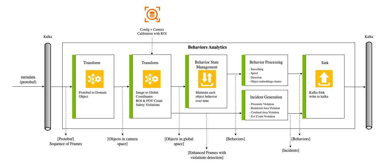
The metadata from the perception layer represents a frame containing object detection bounding boxes, tracking IDs, embedding vectors, and other attributes. This input is processed by the pipeline to generate Behavior data. A Behavior represents an object tracked over time with its associated attributes. The key components of the pipeline are:

• Protobuf Message to Frame: Converts protobuf messages or byte arrays into Frame objects.

• Dynamic Calibration: Loads and manages calibration data, supporting multiple coordinate systems (image, Cartesian, geo) and monitoring for calibration file changes.

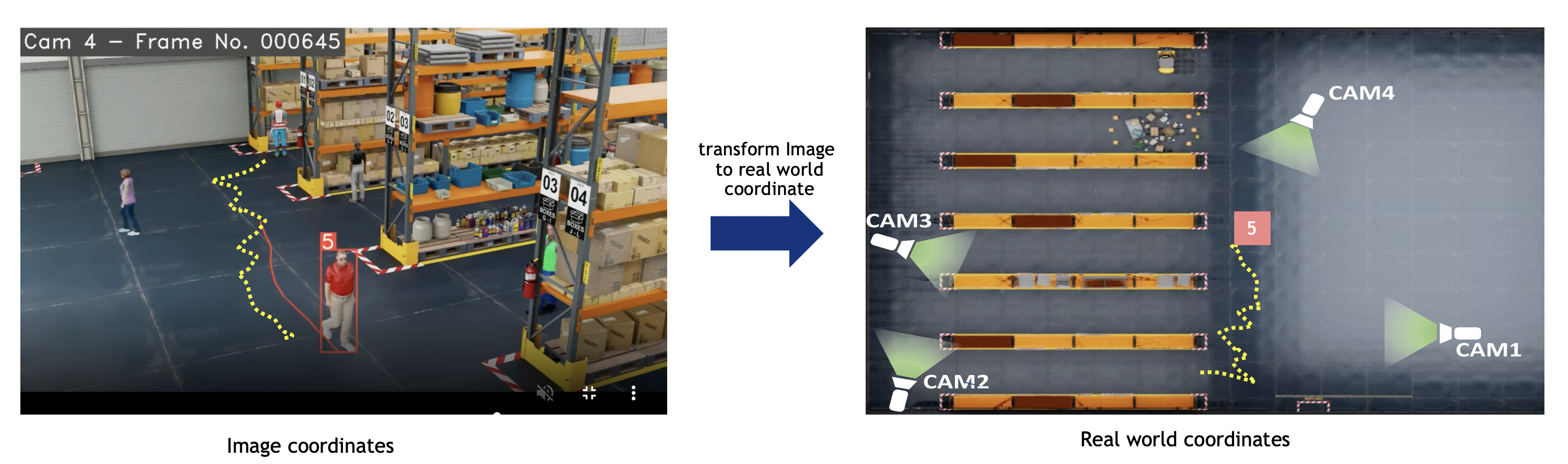
• Image to Real World Coordinate: Transforms image coordinates to real-world coordinates (latitude, longitude) or other coordinate systems such as Cartesian. Also validates if points fall within defined Regions of Interest (ROI).

• Behavior State Management: Manages the state of each object’s Behavior for individual cameras, processing objects across all camera sensors simultaneously.

• Behavior Processing: Calculates key metrics such as speed, direction, and distance based on object movement, appearance, and embeddings.

• Video Embedding Downsampling: Optional. Compresses time-series video embedding data (e.g. VisionLLM) per sensor while preserving patterns and transitions; supports Swinging Door Trending (SDT) and Sliding Window algorithms.

• Event Detection: Generates events including Tripwire events and ROI events.

• Incident Generation: Detects violations (proximity, restricted zone, confined zone, FOV count) and generates incidents when violations persist beyond configured thresholds.

• Sink: Sends Behavior data, events, and incidents to message brokers (Kafka, Redis Streams, or MQTT).

Input & Output

The pipeline stages and their corresponding inputs and outputs are shown below:

Each stage’s inputs and outputs:

Transform	Input (source)	Output (sink)	Description
Protobuf to Frame Object	Protobuf (Kafka)	Dataset of Frame Object	Converts Protobuf bytes to Dataset of frames
Image to Geo Coordinates	Dataset + Calibration	Dataset with Geo Coordinates	Perspective Transform using camera
Calibration ROI Check	Dataset + ROI	Filtered Dataset	Point in Polygon
Behavior State Management	Dataset	Dataset of Behavior (backed up by persistence storage)	Maintains state of Behavior for multiple moving objects
Behavior Processing	Dataset of Behavior + Configuration	Dataset of Behavior with enriched features	Computes Length/Speed/Direction, Object embeddings cluster
Sink: Kafka Sink	Dataset of Frame	Protobuf (Kafka)	Sends dataset to Kafka
Tripwire/ROI Events	Dataset of Behavior + Tripwire/ROI Definition	Tripwire/ROI Events	Generates trip events when a Person/Object crosses a tripwire Generates ROI events when a Person/Object enter/exit a ROI.
ROI + FOI Count Proximity/Zone Violation	Dataset of frames	enhanced Frames	Counts objects in ROI and FOV by type Detects proximity and zone violations based on object distance
Incident Generation	Enhanced Frames with Violations	Incidents	Tracks violations over time and generates incidents when they persist beyond configured thresholds

Configuration

ConfigFile

The configuration file supports multiple message broker types. You can configure Kafka, Redis Streams, or MQTT based on your deployment requirements. Set sourceType and sinkType in the app section to specify which broker to use (default is kafka).

{
   "kafka": {
     "brokers": "localhost:9092",
     "consumer": {
       "autoOffsetReset": "latest",
       "enableAutoCommit": false,
       "maxPollIntervalMs": 900000,
     "maxPartitionFetchBytes": 10485760,
     "fetchMaxBytes": 104857600,
       "maxPollRecords": 10000,
     "timeout": 0.01
     },
     "producer": {
       "lingerMs": 0
     },
   "topics": [
     {"name": "raw", "value": "mdx-raw"},
     {"name": "frames", "value": "mdx-frames"},
     {"name": "behavior", "value": "mdx-behavior"},
     {"name": "notification", "value": "mdx-notification"},
     {"name": "events", "value": "mdx-events"},
     {"name": "incidents", "value": "mdx-incidents"}
   ]
   },
   "redisStream": {
     "host": "localhost",
     "port": 6379,
   "consumer": {
     "readCount": 8,
     "readBlockMs": 4
   },
   "producer": {
     "maxLen": 10000
   },
   "group": "mdx-app",
     "streams": [
       {"name": "raw", "value": "mdx-raw"},
       {"name": "behavior", "value": "mdx-behavior"},
     {"name": "notification", "value": "mdx-notification"},
       {"name": "incidents", "value": "mdx-incidents"}
   ]
   },
   "mqtt": {
     "host": "localhost",
     "port": 1883,
   "clientId": "mdx-app",
   "keepAliveSec": 60,
   "consumer": {
     "qos": 1,
     "maxPollCount": 16,
     "pollTimeoutSec": 1
   },
   "producer": {
     "qos": 1,
     "retain": true
   },
   "topics": [
     {"name": "raw", "value": "mdx-raw"},
     {"name": "behavior", "value": "mdx-behavior"},
     {"name": "notification", "value": "mdx-notification"},
     {"name": "incidents", "value": "mdx-incidents"}
   ]
   },
   "sensors": [
     {
       "id": "default",
       "configs": [
       {"name": "proximityDetectionEnable", "value": "true"},
       {"name": "proximityDetectionThreshold", "value": "1.8"},
       {"name": "proximityDetectionCenterClasses", "value": "[\"Person\"]"},
       {"name": "proximityDetectionSurroundingClasses", "value": "[\"Person\"]"}
       ]
     }
   ],
   "app": [
   {"name": "behaviorWatermarkSec", "value": "30"},
   {"name": "behaviorStateTimeout", "value": "10"},
   {"name": "behaviorMaxPoints", "value": "200"},
   {"name": "objectConfidenceThreshold", "value": "0.5"},
   {"name": "sourceType", "value": "kafka"},
   {"name": "sinkType", "value": "kafka"},
   {"name": "numWorkersForBehaviorCreation", "value": "2"},
   {"name": "numWorkersForFrameEnhancement", "value": "2"},
   {"name": "proximityViolationIncidentEnable", "value": "true"},
   {"name": "proximityViolationIncidentThreshold", "value": "1"},
   {"name": "proximityViolationIncidentExpirationWindow", "value": "1"},
   {"name": "restrictedAreaViolationIncidentEnable", "value": "true"},
   {"name": "restrictedAreaViolationIncidentThreshold", "value": "1"},
   {"name": "restrictedAreaViolationIncidentExpirationWindow", "value": "1"},
   {"name": "confinedAreaViolationIncidentEnable", "value": "true"},
   {"name": "confinedAreaViolationIncidentThreshold", "value": "1"},
   {"name": "confinedAreaViolationIncidentExpirationWindow", "value": "1"},
   {"name": "fovCountViolationIncidentEnable", "value": "true"},
   {"name": "fovCountViolationIncidentObjectThreshold", "value": "3"},
   {"name": "fovCountViolationIncidentThreshold", "value": "1"},
   {"name": "fovCountViolationIncidentExpirationWindow", "value": "1"},
   {"name": "fovCountViolationIncidentObjectType", "value": "Person"}
   ]
 }

Configuration Parameters

• Message Broker Selection: The pipeline supports multiple message brokers. Configure sourceType and sinkType in the app section:

  • kafka (default): Use Kafka for message streaming

  • redisStream: Use Redis Streams for lightweight deployments

  • mqtt: Use MQTT for IoT-oriented deployments

• Kafka Broker: Configure Kafka connection for message streaming:

  • brokers: List of broker host:port pairs (e.g., 10.137.149.51:9092). The sensor-processing layer sends all metadata to this Kafka broker, and the Python streaming pipeline consumes the metadata.

  • consumer.autoOffsetReset: Where to start reading when no offset exists (default: earliest)

  • consumer.enableAutoCommit: Enable automatic offset commits (default: false)

  • consumer.maxPollIntervalMs: Maximum delay between poll invocations in milliseconds (default: 900000)

  • consumer.maxPartitionFetchBytes: Maximum bytes per partition per fetch request (default: 10485760)

  • consumer.fetchMaxBytes: Maximum bytes per fetch request (default: 104857600)

  • consumer.maxPollRecords: Maximum records returned per poll (default: 10000)

  • consumer.timeout: Consumer timeout in seconds (default: 0.01)

  • producer.lingerMs: Time to wait before sending a batch in milliseconds (default: 0)

  • topics: List of key-value pairs mapping logical names to actual topic names (see table below)

• Redis Stream: Configure Redis connection for Redis Streams-based messaging:

  • host: Redis server hostname (default: localhost)

  • port: Redis server port (default: 6379)

  • db: Redis database number (default: 0)

  • consumer.group: Consumer group name for stream consumption

  • consumer.block: Block timeout in milliseconds for stream reads

  • streams: List of key-value pairs mapping logical names to actual stream names (see table below)

• MQTT: Configure MQTT broker connection:

  • host: MQTT broker hostname

  • port: MQTT broker port (default: 1883)

  • clientId: Client identifier for MQTT connection

  • topics: List of key-value pairs mapping logical names to actual topic names (see table below)

• Topics/Streams: Each entry is a key-value pair where name is the logical key used by the pipeline and value is the actual topic or stream name:

  Topic/Stream Mappings

  Key (name)	Default Value (value)	Description
  raw	mdx-raw	Comma-separated list of topics. The sensor-processing layer sends metadata to this topic. Multiple topics may be needed when the tracker is switched off for some sensors in the sensor-processing layer (DeepStream) and run externally.
  behavior	mdx-behavior	All behavior data is sent to this topic by the Python streaming pipeline. See Behavior Processing.
  events	mdx-events	All events, including tripwire and ROI events, are sent to this topic by the Python streaming pipeline.
  frames	mdx-frames	Enriched frames metadata. The pipeline may or may not use this topic.
  notification	mdx-notification	Notifications such as calibration updates, sensor additions, or deletions.
  spaceUtilization	mdx-space-utilization	Space utilization data. The pipeline may or may not use this topic.
  incidents	mdx-incidents	Incident data from the analytics pipeline when violations persist beyond configured thresholds.
  behaviorPlus	mdx-behavior-plus	Enhanced behavior data (Smart Cities Application).
  anomaly	mdx-alerts	Anomaly detection alerts (Smart Cities Application).

• App Pipeline Config

  • numWorkersForBehaviorCreation: Number of workers to run behavior creation. If set to 0, behavior creation will not run. Required (no default)

  • numWorkersForFrameEnhancement: Number of workers to run frame enhancement. If set to 0, frame enhancement will not run. Required (no default)

  • in3dMode: If true, the pipeline runs in 3D mode. Default: false

  • compactFrame: If true, the pipeline compacts the frame metadata. Default: false

  • objectConfidenceThreshold: Minimum confidence score for object detection. Objects below this threshold are filtered out. Default: 0.5

  • clusterThreshold: Cosine similarity threshold for embedding clustering. Default: 0.9

  • imageLocationMode: (Image calibration only.) Bbox reference point: bottom_center or center. Default: bottom_center

• Tripwire (Sensor-level config)

  • tripwireMinPoints: Minimum number of points an object must be detected before and after the tripwire to generate a trip event. Default: 5

• Proximity Detection (Sensor-level config)

  • proximityDetectionEnable: If true, the pipeline checks for proximity violations between objects. Default: false

  • proximityDetectionThreshold: Distance threshold (in meters) for proximity detection. Default: 1.8

  • proximityDetectionCenterClasses: List of object types to use as center objects for proximity detection (e.g., AMR, humanoid). Default: []

  • proximityDetectionSurroundingClasses: List of object types to check proximity against the center objects. Default: []

• State Management

  • behaviorStateTimeout: If an object is not detected or the frame message arrives late for a configurable period (in seconds), the object state will be deleted from memory and disk. If an object with the same id is sent again, a new behavior will be created. The uniqueness of the behavior is based on sensor + id + start timestamp. Default: 10

  • behaviorStateValidInterval: Minimum time interval (in seconds) for a behavior to be considered valid. Default: 6

  • behaviorWatermarkSec: The watermark for the behavior in seconds. Default: 30

  • behaviorMaxPoints: Maximum number of behavior points to store. Default: 200

  • stateManagementFilter: Only object types in this list will be managed by state management; other object types will be ignored. If the list is empty, all object types will be managed. Default: []

• Frame Management (Sensor-level config)

  • sensorMinFrames: Minimum number of frames to process for frame state management. Default: 5

• Video Embedding (App-level config)

  • embedEnableDownsampling: If true, enable video embedding downsampling; if false, embeddings are passed through unchanged. Default: false

  • embedDownsamplerType: Downsampler algorithm: sdt or window. Default: window

  • embedSensorTTLSec: Seconds of inactivity after which a sensor’s downsampler state is purged. Default: 3600

  • embedDownsampleToleranceMode: Tolerance metric: distance or cosine. Default: cosine

  • embedDownsampleSimilarityThreshold: Cosine similarity threshold (cosine mode). Default: 0.90

  • embedDownsampleDistanceThreshold: Euclidean distance threshold in normalized space (distance mode). Default: 0.15

  • embedDownsampleMaxIntervalSec: Maximum interval (seconds) between saved points; forces a save if exceeded. Default: 60

  • embedDownsampleWindowSize: Sliding window size in points (window algorithm only). Default: 60

  • embedDownsampleMinNeighbours: Minimum consecutive similar neighbors to skip a point (window algorithm only). Default: 3

• Space Analytics

  • spaceAnalyticsIntervalSec: Interval (in seconds) to invoke space analytics. Default: 5.0

  • spaceAnalyticsGridSize: Size of the grid for space analytics. The target area is treated as a rectangle and divided into smaller square grids. The grid size is the length of one side of the square grid. Pallet placement is based on the grids. Smaller grid sizes increase the search space. Default: 0.2

  • spaceAnalyticsUnsafeSize: Size threshold (in meters) to determine unsafe pallets. If a pallet is placed partially outside the designated area (buffer zone) and the size of the outside portion exceeds this value, it is flagged as unsafe. Default: 0.5

  • spaceAnalyticsTargetClasses: List of object types to target for space analytics. Default: [“Box”, “Pallet”]

  • spaceAnalyticsUseGA: If true, the pipeline uses a genetic algorithm to optimize object placements for maximum space utilization; otherwise, a greedy search algorithm is used. Default: false

  • spaceAnalyticsPopulationSizeGA: Population size for the genetic algorithm. Effective only if useGA is true. Default: 200

  • spaceAnalyticsNumGenerationsGA: Number of generations for the genetic algorithm. Effective only if useGA is true. Default: 300

• Playback Configs

  • playbackSensors: List of sensor IDs to include in playback. If empty, all sensors are used. Default: []

  • playbackLoop: Number of times to loop through playback data. Default: 1

  • playbackFilterEmptyObjects: If true, filters out frames with no objects. Default: true

  • playbackInSimulationMode: If true, uses simulated time for playback. Default: false

  • playbackStartUpDelaySec: Delay in seconds before playback starts. Default: 0

  • playbackSimulationTimedeltaInMin: Time delta in minutes for simulation mode. Default: 60

  • playbackSimulationFps: Frames per second for simulation playback. Default: 1

  • playbackSimulationBaseTime: Base timestamp for simulation (ISO format). Default: “”

• Trajectory Configs (Smart Cities Application)

  • trajGeoCoordEnable: Enable geo coordinates for trajectory processing. Default: true

  • trajDirectionMode: Direction calculation mode (0=bearing-based). Default: 0

  • trajDirectionClusterMode: Direction clustering mode. Default: 1

  • trajSmoothMinPoints: Minimum points required for trajectory smoothing. Default: 20

  • trajSmoothWindowSize: Window size for trajectory smoothing. Default: 5

  • trajDistanceStride: Stride for distance computation. Default: 5

  • trajSpeedSegmentSize: Segment size for speed computation. Default: 10

  • mapMatchingMaxPoints: Maximum points for map matching. Default: 5

  • mapMatchingClasses: Object classes to apply map matching. Default: []

• Anomaly Detection (Sensor-level config, Smart Cities Application)

  • anomalyIgnoreSensors: List of sensor IDs to ignore for anomaly detection. Default: []

  • anomalyClasses: List of object classes for anomaly detection. Default: []

  • anomalySpeedViolation: JSON config for speed violation detection. Includes enable, mphThreshold, timeIntervalSecThreshold.

  • anomalyUnexpectedStop: JSON config for unexpected stop detection. Includes enable, mphThreshold, timeIntervalSecThreshold.

  • anomalyAbnormalMovement: JSON config for abnormal movement detection. Includes enable, distanceMetersThreshold, timeIntervalSecThreshold, changeInDirectionDegree.

  • anomalyCollisionDetection: JSON config for collision detection. Includes enable, targetClasses, distanceMetersThreshold.

• Inference Config

  • inference.enable: Enable Triton Inference Server integration. Default: false

  • inference.url: URL of the Triton Inference Server. Default: localhost:8000

• Overriding Default Config

  • All sensors use the configuration defined with sensor “id”: “default”.

    {
      "sensors": [
        {
          "id": "default",
          "configs": [
              ...
          ]
       },
       ...
    }
    

  • You can override one or more default configurations for a given sensor by adding a new entry with the sensor name. Configuration keys in JSON use camelCase (e.g. tripwireMinPoints). The following overrides the default tripwire min points for sensor-id Warehouse_Cam1:

      {
        "sensors": [
        {
            "id": "default",
            "configs": [
                ...
            ]
        },
        {
            "id": "Warehouse_Cam1",
            "configs": [
                {
                    "name": "tripwireMinPoints",
                    "value": "11"
                },
                ...
            ]
          }
        ]
      }
    

CalibrationFile

Use the Calibration tool to generate the JSON file. For more details, refer to the Calibration. For the calibration JSON structure, see Calibration Schema.

Components & Customization

To help understand more and potentially customize the microservice, here’s a deep dive of the components’ implementation and the data flow between them:

Application Framework

The recommended way to build analytics applications is using the BaseApp framework. When you build a new pipeline (by modifying ours or creating one from scratch), the library dependencies will be fetched from our artifact repository.

BaseApp provides:

• Automatic source/sink management for multiple message broker types (Kafka, Redis Streams, MQTT)

• Worker-based multi-processing with configurable parallelism

• Dynamic calibration support with automatic type detection (image, cartesian, geo)

• Graceful shutdown handling with signal handlers (SIGINT, SIGTERM)

• Performance monitoring with BatchStats

• Built-in write methods for behaviors, events, frames, incidents, and anomalies

Example

from mdx.analytics.core.app.app_base import BaseApp
from mdx.analytics.core.app.app_runner import run

class MyApp(BaseApp):

    def __init__(self, config, calibration_path):
        super().__init__(config, calibration_path)
        self.register_processor(self.read_raw, self.process, num_workers=2)

    def process(self, frames, stats):
        enhanced = [self.calibration.transform_frame(f) for f in frames]
        self.write_frames(enhanced)

if __name__ == '__main__':
    run(MyApp)

For a complete example, refer to apps/spatial_analytics/main_spatial_analytics_2d_app.py.

Built-in Methods

BaseApp Methods

Method	Description
read_raw(group_id_suffix)	Read raw frame data from the configured source (Kafka/Redis/MQTT)
read_behavior(group_id_suffix)	Read behavior data from the source
read_events(group_id_suffix)	Read event data from the source
read_anomaly(group_id_suffix)	Read anomaly data from the source
write_frames(frames)	Write enhanced frame data to the sink
write_behaviors(behaviors)	Write behavior data to the sink
write_events(events)	Write event data to the sink
write_incidents(incidents)	Write incident data to the sink
write_anomalies(anomalies)	Write anomaly data to the sink
write_space_utilization(output)	Write space utilization data to the sink
write_behaviors_with_clustering(behaviors)	Write behaviors with trajectory clustering to behaviorPlus topic
register_processor(poller, handler, num_workers)	Register a processing handler with specified worker count
close()	Clean up resources (source, sink, calibration)

Protobuf to Object

The protobuf message payload is sent to a message broker (Kafka, Redis Streams, or MQTT) as a ByteArray. For example, a Kafka ProducerRecord contains (topic, key, value), with topic=mdx-raw, key=sensor-id, and value=protobuf-byte-array. When the Behavior Analytics microservice receives the message, it transforms the byte array into a Frame object. The Frame object corresponds to the video frame being processed by the perception layer. It contains all detected objects for a given frame and their corresponding bounding boxes in a single message. Each object may include additional attributes like embedding vectors, pose data, etc.

To read more about the schema, refer to the Protobuf Schema.

Usage

When using the BaseApp framework, data reading is handled automatically via self.read_raw():

from mdx.analytics.core.app.app_base import BaseApp
from mdx.analytics.core.schema.proto import schema_pb2 as nvSchema
from mdx.analytics.core.utils.processing_stats import BatchStats

class MyApp(BaseApp):
    def __init__(self, config, calibration_path):
        super().__init__(config, calibration_path)
        self.register_processor(self.read_raw, self.process, num_workers=2)

    def process(self, frames: list[nvSchema.Frame], stats: BatchStats) -> None:
        # frames are automatically deserialized from protobuf
        for frame in frames:
            print(f"Frame {frame.id} from sensor {frame.sensorId}")

For standalone source usage (without BaseApp), use the source factory:

from mdx.analytics.core.stream.source.source_factory import get_source
from mdx.analytics.core.stream.source.source_base import StreamMessageProtoDeserializer
from mdx.analytics.core.schema.proto import schema_pb2 as nvSchema
from mdx.analytics.core.schema.config import AppConfig

# Load config and create source based on sourceType (kafka/redisStream/mqtt)
config = AppConfig(**config_data)
source = get_source(config)

# Poll raw frames from the source
frames = source.poll(
    src_key="raw",
    msg_deserializer=StreamMessageProtoDeserializer(nvSchema.Frame)
)

Definition

The raw frame object is translated to JSON before being stored in Elasticsearch, the JSON representation is as below.

{
  "version": "4.0",
  "id": "252",
  "timestamp": "2022-02-09T10:45:10.170Z",
  "sensorId": "xyz",
  "objects": [
    {
      "id": "3",
      "bbox": {
        "leftX": 285.0,
        "topY": 238.0,
        "rightX": 622.0,
        "bottomY": 687.0
      },
      "type": "Person",
      "confidence": 0.9779,
      "info": {
        "gender": "male",
        "age": 45,
        "hair": "black",
        "cap": "none",
        "apparel": "formal"
      },
      "embedding": {
        "vector": [
          1.4162299633026123,
          -0.28852298855781555,
          1.1123499870300293,
          -0.047587499022483826,
          -2.293760061264038,
          0.8388320207595825
        ]
      }
    }
  ]
}

API

BaseApp provides the following read methods that internally use the configured source:

# BaseApp read methods (use these when extending BaseApp)
class BaseApp:
    # Read raw frames from the configured source
    # group_id_suffix is used when multiple processors read from the same topic
    def read_raw(self, group_id_suffix: str | None = None) -> list[nvSchema.Frame]

    # Read behavior data from the source
    def read_behavior(self, group_id_suffix: str | None = None) -> list[Behavior]

    # Read event data from the source
    def read_events(self, group_id_suffix: str | None = None) -> list[Behavior]

    # Read anomaly data from the source
    def read_anomaly(self, group_id_suffix: str | None = None) -> list[Behavior]

For low-level source access, use the Source interface:

# Source base class interface
class Source:
    # Poll and deserialize messages from a source
    def poll(
        self,
        src_key: str,                    # Stream key (e.g., "raw", "behavior")
        msg_deserializer: Callable,      # Function to deserialize messages
        group_id_suffix: str | None = None
    ) -> list[Any]

    # Read raw stream messages (before deserialization)
    def read(
        self,
        src_key: str,
        group_id_suffix: str | None = None
    ) -> list[StreamMessage]

    # Close the source and release resources
    def close(self) -> None

Image to Global Coordinate Transformation

Frame metadata includes object-id, bbox in image/pixel coordinates, object-type, and other attributes.

Cartesian or geo calibration: Diagram: image coordinates (left) transformed via homography to real-world—geo (lat/lon) or Cartesian (meters)—for speed, distance, ROI, etc. Bbox reference is configurable for image calibration (see Image calibration (no transformation)).

Image calibration: No transformation; output stays in image/pixel. Default when no calibration file or calibrationType is "image".

Usage

With BaseApp, calibration is initialized as self.calibration. DynamicCalibration detects type (image, cartesian, geo) from the JSON and creates the right implementation.

from mdx.analytics.core.app.app_base import BaseApp
from mdx.analytics.core.utils.schema_util import nv_frame_to_messages

class MyApp(BaseApp):
    def process(self, frames, stats):
        # self.calibration is automatically initialized (DynamicCalibration)
        # Filter frames to only include sensors defined in calibration
        frames = self.calibration.filter_frames_by_sensor_id(frames)

        # Transform frames to enhanced frames (with real world coordinates, ROI/FOV count, violations)
        enhanced_frames = [self.calibration.transform_frame(frame) for frame in frames]

        # For behavior processing, convert frames to messages
        messages = [
            msg for frame in frames
            for msg in nv_frame_to_messages(frame, object_filter=self.config.state_mgmt_filter)
        ]
        # Transform messages with calibration (updates locations)
        updated_messages = [self.calibration.transform(msg) for msg in messages]

For standalone usage without BaseApp:

from mdx.analytics.core.transform.calibration.calibration_dynamic import DynamicCalibration
from mdx.analytics.core.schema.config import AppConfig

config = AppConfig(**config_data)
calibration = DynamicCalibration(config, calibration_path)
calibration.start_listen()  # Start monitoring for calibration file changes

# Transform frames
enhanced_frames = [calibration.transform_frame(frame) for frame in frames]

Calibration types

Three types are supported, selected by calibrationType in the calibration JSON (defaulting to image when no file is provided). See the subsections below.

Image calibration (no transformation)

CalibrationI does not transform coordinates; output stays in image/pixel space (no homography). Use when:

• No calibration file at startup (or one will be added later)

• calibrationType is "image"

• Analytics are image-space only

No homography; transform_bbox returns the chosen bbox reference point. 2D bbox only; 3D not supported. filter_frames_by_sensor_id returns all frames (no sensor filtering).

Image location mode (image calibration only)

Config imageLocationMode (JSON key: imageLocationMode) sets the bbox reference point:

Image location mode

Value	Description
bottom_center (default)	Center of bbox bottom edge (center X, bottom Y). Best for ground-plane/foot.
center	Bbox center (center X, center Y).

Applies only to image calibration (CalibrationI). Cartesian/geo use a fixed convention.

Euclidean/Cartesian calibration

CalibrationE transforms image coordinates to real-world Cartesian (meters) via a per-sensor homography matrix. Use for building or floor maps. Supports 2D bbox (bottom-center reference) and 3D bbox when in3dMode is true; transform_bbox uses perspective transform. Frames are filtered by sensor ID (only sensors defined in calibration are kept).

Geo calibration

Calibration transforms image coordinates to real-world; output is lat/lon (WGS-84) or Cartesian depending on config (trajGeoCoordEnable, coordinate reference system, origin). Handles four cases: latlon→latlon, latlon→cartesian, cartesian→latlon, cartesian→cartesian. 2D bbox only (bottom-center); homography from image to geo/cartesian. Frames are filtered by sensor ID.

Definition

Message represents a single object + contextual data:

class Message(BaseModel):
  messageid: str  # Unique identifier for the message, sensorId + "#-#" + objectId
  timestamp: datetime  # Timestamp of the message
  sensor: Sensor  # Sensor metadata
  object: Optional[Object] = None  # Object metadata
  mdsversion: str = ""  # Version
  place: Place = Field(default_factory=Place)  # Place metadata
  analyticsModule: Optional[AnalyticsModule] = None  # Analytics module that processed the message
  event: Optional[Event] = None  # Event information associated with the message
  videoPath: str = ""  # Video path

API

# Checks if the given point falls within the ROI for the given sensor and roi_id.
def point_in_polygon(self, point: Coordinate | Point2D | nvSchema.Coordinate | nvSchema.Point2D, sensor_id: str, roi_id: str) -> bool

# Transform 4 corners of bbox image coordinates to a single real world coordinates based
# on Homography Matrix for a given sensor-id
# Also transform real world coordinates (cartesian) to lat-lon, with respect
# to a given origin. The transformation matrix and the origin are initialized
# from an external configuration if transformation matrix is not present, it will return image coordinates
def transform_bbox(self, bbox: Bbox, sensor_id: str) -> Tuple[Coordinate, Location]

# Transform 8 corners of 3D bbox real world coordinates to a single real world coordinates
# Also transform real world coordinates (cartesian) to lat-lon, with respect to a given origin.
# Transformation matrix is not required for 3D bbox.
def transform_bbox3d(self, bbox: Bbox, sensor_id: str) -> Tuple[Coordinate, Location]

# Transform the message to a new message with updated location in real world coordinates
# Internally invokes transform_bbox/transform_bbox3d and Returns updated Message
def transform(self, msg: Message) -> Message

# Transform the raw frame to enhanced frames (with object locations in real world coordinates, ROI/FOV count, zone violations, etc.)
# Internally invokes transform_bbox/transform_bbox3d and Returns updated Frame
def transform_frame(self, frame: nvSchema.Frame) -> nvSchema.Frame

Behavior State Management (BSM)

As the perception layer tracks a given object, the object-id remains the same during the time the object is seen by a single camera. This helps in forming a Behavior for a given object. Behavior defines the sequence of real world coordinates an object was detected at, its appearance, embeddings, pose etc., The span of the Behavior may be short lived based on how long it was seen with respect to a given camera. There are cases where the span of the Behavior can be very long. An example is a car stopped due to a red signal or a car parked on the roadside or a person standing in a queue.

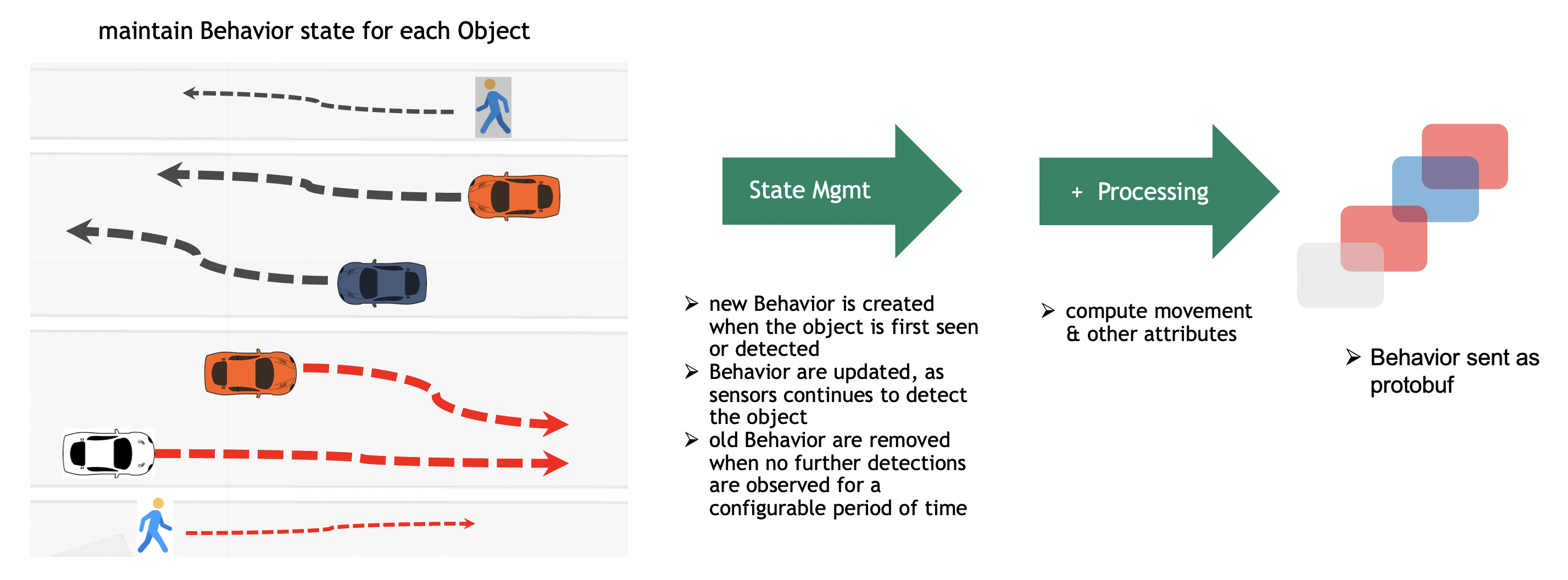
The above diagram depicts a few tracks with respect to vehicle and people movement as seen by the camera. However, this can be any kind of object, like a robot, a bicycle, etc. The BSM maintains the Behavior state on live streaming data. As the objects are detected by the perception layer and frame metadata is sent over the network to the Kafka broker, the Behavior Analytics pipeline consumes all detections corresponding to an object and maintains the Behavior state in memory. The in-memory copy of the Behavior is backed up by a persistent store for reliability. The Behavior gets updated when the perception layer sends more detection metadata with respect to the same object. At some point in time, the object gets out of the Field of View of the camera and no more metadata is sent to the BSM. The BSM then cleans up the Behavior corresponding to the object that is no longer seen. The period of time after which the BSM cleans up the state is configurable. To keep the memory footprint of the Behavior state low, only minimal information is stored during the life of the Behavior. The state comprises the object ID, sensor ID, locations, start and end timestamps, object embeddings, etc.

Behavior State Management API

Usage

from mdx.analytics.core.stream.state.behavior.state_management_e import StateMgmtE, StateMgmtEWithTripwire
from mdx.analytics.core.utils.schema_util import messages_to_map

# Initialize state management with config and calibration
state_mgmt = StateMgmtEWithTripwire(config, calibration)

# Convert messages to map: key = sensorId + "#-#" + objectId
messages_map = messages_to_map(updated_messages)

# Process messages and get behaviors + trip events
behaviors, events = [], []
for message_key, msgs in messages_map.items():
    behavior, trip = state_mgmt.update_behavior(message_key=message_key, messages=msgs)
    if behavior:
        behaviors.append(behavior)
    if trip:
        # Use trip for tripwire/ROI event detection
        events.extend(tripwire_event.get_events(trip))
        events.extend(roi_event.get_events(trip))

# For behavior only (no trip events), use StateMgmtE
state_mgmt_simple = StateMgmtE(config, calibration)
behavior = state_mgmt_simple.update_behavior(message_key, msgs)  # Returns Behavior | None

Definition

class ObjectState(BaseModel):

  id: str  # Unique identifier for the object, sensorId + "#-#" + objectId
  start: datetime  # Start timestamp of the object state
  end: datetime  # End timestamp of the object state
  points: List[Coordinate] = Field(default_factory=list)  # Sequence of points' coordinates
  sampling: int = 1  # Sampling rate
  lastXpoints: List[Coordinate] = Field(default_factory=list)  # Last X points of the object state without sampling
  object: Optional[Object] = None  # Object metadata
  objectTypeScoreSumMap: Optional[Dict[str, float]] = None  # Object type to confidence score sum map
  model: Optional[Model] = None  # Model including clustered embeddings

API

from mdx.analytics.core.stream.state.behavior.state_management_e import StateMgmtE, StateMgmtEWithTripwire

class StateMgmtEWithTripwire:
    """State management with tripwire event support."""

    def __init__(self, config: AppConfig, calibration: CalibrationBase) -> None:
        """Initialize with config and calibration."""

    def update_behavior(
        self,
        message_key: str,
        messages: list[Message],
        **kwargs
    ) -> tuple[Behavior | None, Behavior | None]:
        """
        Update behavior state and return (behavior, trip_behavior).
        - behavior: Full behavior for storage/analysis
        - trip_behavior: Tracklet for tripwire/ROI event detection
        """

class StateMgmtE(StateMgmtEWithTripwire):
    """State management without tripwire (simpler API)."""

    def update_behavior(
        self,
        message_key: str,
        messages: list[Message],
        **kwargs
    ) -> Behavior | None:
        """Update behavior state and return behavior only."""

Note

When using BaseApp, use the built-in write_behaviors() and write_events() methods to publish results. See Sink.

Embeddings Cluster

Behavior comprises of sequence of real world coordinates an object was detected at, its appearance, embeddings, pose etc., The embeddings or the feature vector represents the object appearance, these embeddings are generated continuously and may vary based on factors like lighting, camera angle and field of view. Embeddings cluster tries to summarize 100s of feature vectors into few salient ones that can be used to represent an object appearance. The cluster algorithm used is CRP, it is a non-parametric generative Bayesian model, the data is processed in a streaming mode, clustering is done in an incremental model. As the sequence of embeddings is processed by the pipeline, it simultaneously learns the number of clusters, the model of each cluster, and entity assignments into clusters. The state of the cluster model is maintained by computing the cluster centers across every micro batch.

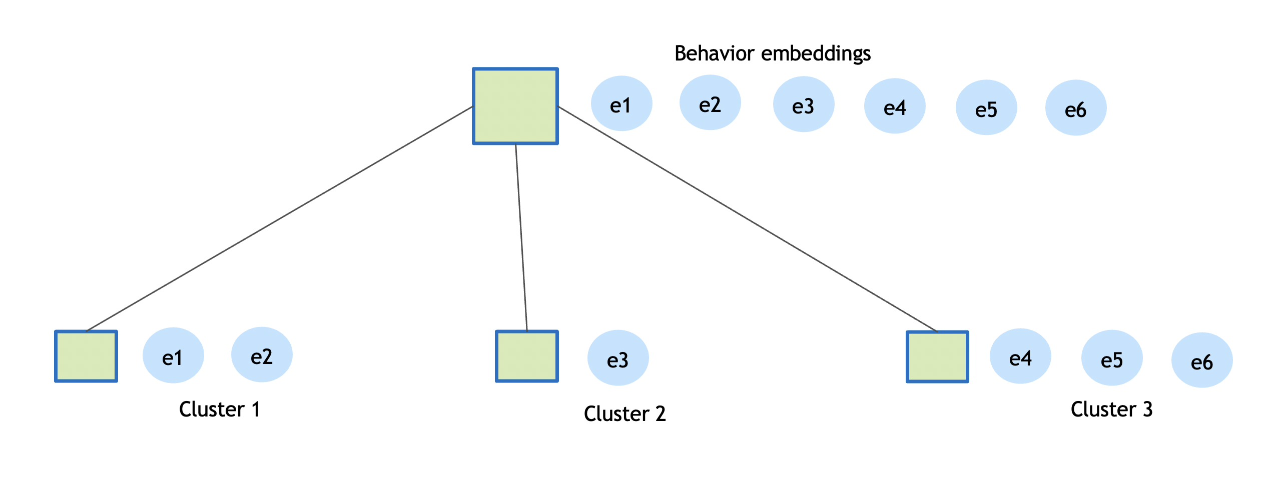
The diagram above shows only a few embeddings instead of hundreds; the idea is to create a few representative embeddings from all the detections for a given object. The clustering distance used is cosine similarity, and the default threshold is 0.9. The clustering process completes when an object is no longer detected by a sensor.

Usage

from mdx.analytics.core.utils.crp import CRP


# Given a list of normalized vectors create the CRP cluster model.
# default pnew=0.9, threshold for creation of new cluster
# if given a new vector is not close enough to any of the existing cluster.
# takes two inputs,  vecs = Array[Embedding], pnew = cosine similarity threshold
model = CRP().cluster(embeddings, cluster_threshold)

# Given a list of normalized vectors and a existing model, create a new CRP cluster model.
# default pnew=0.9, threshold for creation of new cluster
updated_model = CRP().update_model(model, embeddings, cluster_threshold)

Behavior Processing

Behavior Attributes

The key attributes of the Behavior are based on object movement + Object appearance with highest confidence + Sensor + Place + Embeddings + Pose + Gesture + Gaze:

Behavior Attributes

Name	Description
id	unique id of the Behavior, default implementation used <b>sensor-id + object-id. The object-Id is generated by sensor-processing layer. The sensor-processing layer tracks a objects over time and assigns it a unique id. To make the Behavior id unique across all sensors, a combination of sensor-id and object-id is used.
bearing	given two end points of the Behavior represents the initial bearing/direction. Given a sequence of points representing Behavior, the start and end is used as the two endpoints.
direction	represents the direction in which object is moving, bearing is converted to direction like East, West, North or South
distance	in meters, approximate distance computed based on movement of object for each point in the Behavior
linearDistance	Euclidean distance between start and end of Behavior
speed	average speed in miles per hour (mph), computed based on distance traversed over time internal of the Behavior
speedOverTime	speed in miles per hour (mph), The speed computation over time is computed based smaller segments of the Behavior. default is every segment with a span of 1 seconds speed is computed
start	start timestamp in UTC of the Behavior
timeInterval	time span of the Behavior in seconds
locations	representing array of [longitude, latitude] or [x, y]
smoothLocations	representing smoothened array of [longitude, latitude] or [x, y]
edges	The edges represent the road segment of open street map (OSM). Each edge has unique id, road network edges, only applicable for geo coordinates
place	where object was detected
sensor	which detected the object
object	represents type of object and its appearance attributes
event	can be “moving”, “parked”, etc.,
videoPath	URL of the video if stored
embeddings	array of embeddings
pose	array of pose estimations
gesture	array of gesture estimations
gaze	array of gaze estimations

Movement Attributes

For Cartesian coordinates, TrajectoryE is used:

from mdx.analytics.core.schema.trajectory.trajectory_e import TrajectoryE

tr = TrajectoryE(id=state.id, start=state.start, end=state.end, points=state.points)

# compute movement behavior or attributes
tr.bearing
tr.direction
tr.distance
tr.timeInterval
tr.speed
tr.speedOverTime
tr.smoothTrajectory

Note

• For image coordinates use TrajectoryI

• For Geo coordinates use Trajectory

Average Speed Computation

The distance computation is made with respect to two consecutive points in the smoothened trajectory. The trajectory distance is the sum of all the individual distances obtained between consecutive points.

Compute distance d between two consecutive points:

d = √((p1.x - p2.x)^2 + (p1.y - p2.y)^2)

distance = Σd
average_speed = distance / time_interval

Note

For Geo coordinates haversine distance is used.

Speed Computation Over Time

Here is an example of Vehicle moving East with an average speed of 29.95 miles/hr, covering 212.87 meters in 15.90 seconds. However, the average speed may not exactly depict the vehicle speed, how it changes over time. If we consider the speed over time, it looks as below:

speedsOverTime = [35.37, 26.53, 28.63, 30.53, 27.51, 28.34, 29.4, 30.33, 28.79, 26.76, 25.54, 24.71, 23.98, 23.39, 24.32]

The speed computation over time is computed based on smaller segments of the trajectory. default is every segment with a span of 1 seconds speed is computed.

Direction

The Direction is computed based on the bearing of the Object.

The formula is to calculate the bearing of the trajectory from the first to the last point. For Cartesian and image coordinates the angle with the x axis is used.

bearing = math.atan2(p1.y - p2.y, p1.x - p2.x) * 180 / math.pi
bearing = (bearing + 360) % 360

For Cartesian and image coordinates left, right, up & down is used. The direction definition based on bearing is as follows:

# 4-way direction.
directions = ["Right", "Up", "Left", "Down"]
direction = directions[int((bearing / 90) + 0.5) % 4]

Video Embedding Downsampling

Video embedding downsampling reduces the volume of time-series video embedding data (e.g. VisionLLM protobuf messages) while preserving important patterns and transitions. It is useful for pipelines that consume high-dimensional embedding streams and need to store or forward a compressed subset. The implementation supports two algorithms and per-sensor state with configurable tolerance and lifecycle.

Algorithms

• Swinging Door Trending (SDT): Interpolation-based compression. Uses a one-point look-ahead: the last committed point (anchor), a pending point (candidate), and the current point. The candidate is skipped if it lies within a tolerance band of the line from anchor to current. Good for smooth, gradual embedding changes; O(1) memory; one-point latency. Call get_pending_video_embeddings() at shutdown to flush the pending candidate.

• Sliding Window: Neighbor-based novelty detection. Keeps a fixed-size window of recent embeddings; a new point is saved only if it has fewer than min_neighbours consecutive similar neighbors in the window. Good for cyclical or repetitive patterns; O(window size) memory; no look-ahead delay.

Both algorithms support distance (Euclidean in normalized vector space) or cosine (similarity) tolerance metrics. Embeddings are normalized before comparison. Typical thresholds: SDT distance ~0.15, cosine ~0.91; Window distance ~0.45, cosine ~0.90 (looser thresholds for pattern matching).

Configuration

Video embedding is configured via AppConfig.video_embedding (VideoEmbeddingConfig). App-level keys use the embed prefix (camelCase in JSON). For the full list of parameters and defaults, see Configuration Parameters (Video Embedding, App-level config).

Usage

Use VideoEmbeddingStateMgmt with VideoEmbeddingConfig (e.g. from config.video_embedding). Create one manager and call update_video_embeddings(sensor_id, video_embeddings) per sensor for each batch; at shutdown call get_pending_video_embeddings() to flush pending candidates (important for SDT). The class creates downsamplers lazily per sensor and purges sensors inactive beyond sensor_ttl_sec.

from mdx.analytics.core.stream.state.video_embedding.video_embedding_state_mgmt import VideoEmbeddingStateMgmt
from mdx.analytics.core.schema.config import AppConfig
from mdx.analytics.core.utils.schema_util import group_video_embeddings_by_sensor_id

config = AppConfig(**config_data)
state_mgmt = VideoEmbeddingStateMgmt(config.video_embedding)

# Per batch: group by sensor and update
for sensor_id, vid_embeddings in group_video_embeddings_by_sensor_id(video_embeddings).items():
    downsampled = state_mgmt.update_video_embeddings(sensor_id, vid_embeddings)
    # Use downsampled list (e.g. write to sink)

# At shutdown: flush pending (e.g. SDT candidate)
pending = state_mgmt.get_pending_video_embeddings()

Applications such as the fusion search app read video embeddings from a source, pass them through VideoEmbeddingStateMgmt, and write filtered/downsampled results via write_embed_filtered (or a custom sink).

API

from mdx.analytics.core.stream.state.video_embedding.video_embedding_state_mgmt import VideoEmbeddingStateMgmt

class VideoEmbeddingStateMgmt:
    def __init__(self, config: VideoEmbeddingConfig) -> None:
        """Initialize with video embedding config (e.g. AppConfig.video_embedding)."""

    def update_video_embeddings(
        self,
        sensor_id: str,
        video_embeddings: list[nvSchema.VisionLLM]
    ) -> list[nvSchema.VisionLLM]:
        """Process and downsample embeddings for the sensor; returns downsampled list. Skips invalid (no visionEmbeddings)."""

    def get_pending_video_embeddings(self) -> list[nvSchema.VisionLLM]:
        """Flush pending candidates from all sensors (call at shutdown). Critical for SDT."""

Tolerance and algorithm choice can be tuned via the parameters in the Configuration table above.

Event Detection

The event detection system supports two types of events:

• Tripwire Events: It was triggered when objects cross the tripwire line segment.

• ROI Events: It was triggered when objects enter or exit the ROI polygon boundary.

Both tripwire and ROI are defined in the camera/sensor calibration JSON. Multiple tripwires or ROIs can be configured for each sensor.

Tripwire Definition

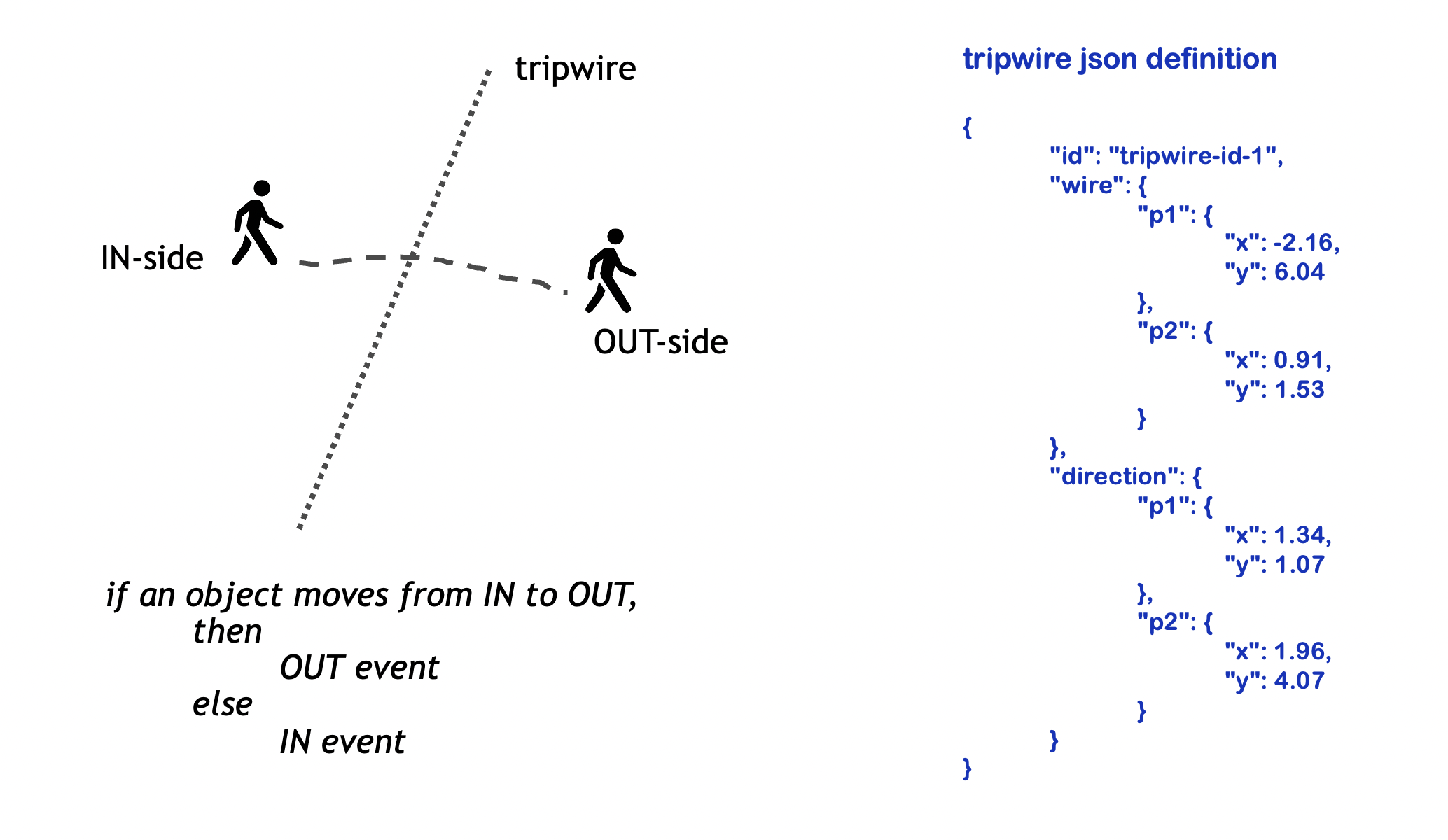
The wire is defined as a line segment between two points. The direction specifies IN point (p1) and OUT point (p2).

ROI Definition

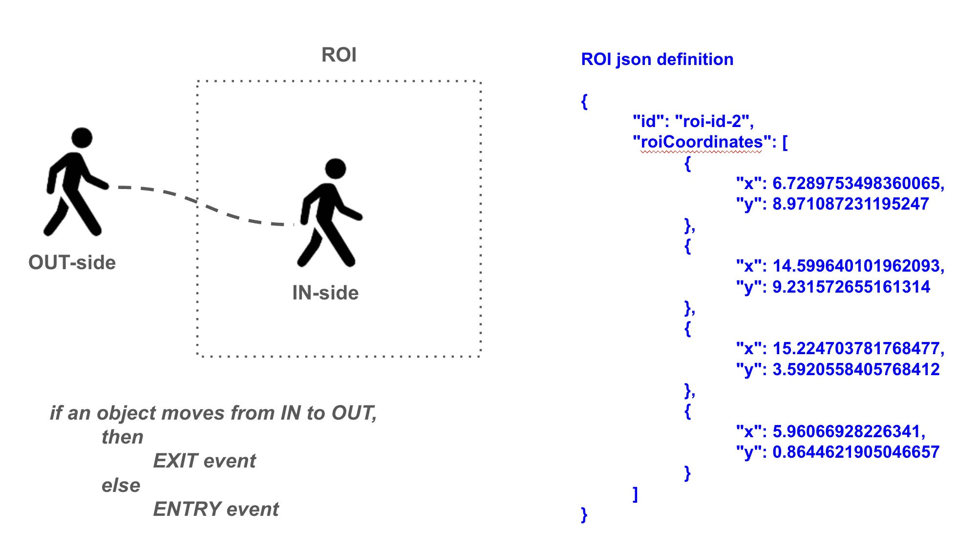
The roiCoordinates define the vertices of the ROI polygon.

Usage

from mdx.analytics.core.app.app_base import BaseApp
from mdx.analytics.core.stream.state.behavior.state_management_e import StateMgmtEWithTripwire
from mdx.analytics.core.transform.event.tripwire_event import TripwireEvent
from mdx.analytics.core.transform.event.roi_event import ROIEvent

class MyApp(BaseApp):
    def __init__(self, config, calibration_path):
        super().__init__(config, calibration_path)
        self.state_mgmt = StateMgmtEWithTripwire(self.config, self.calibration)
        self.tripwire_event = TripwireEvent(self.config, self.calibration)
        self.roi_event = ROIEvent(self.config, self.calibration)

    def process(self, frames, stats):
        # Process messages and get behavior + trip
        behavior, trip = self.state_mgmt.update_behavior(key, msgs)

        # Generate events from trip behavior
        if trip:
            events = self.tripwire_event.get_events(trip)
            events.extend(self.roi_event.get_events(trip))
            self.write_events(events)

Definition

The Behavior object (trip behavior from StateMgmtEWithTripwire) contains the trajectory information including locations, start and end timestamps for each tracked object. The system processes this trajectory by:

1. Splitting it into overlapping tracklets of length minTripLength

2. For tripwires: Checking if tracklets have sufficient points before and after crossing the wire

3. For ROIs: Checking if tracklets have sufficient points both inside and outside the ROI boundary

API

def get_events(self, behavior: Behavior) -> List[Behavior]

Note

For image coordinates use same TripwireEvent, ROIEvent.

Incidents

The Incidents framework detects violations in video frames and tracks them over time to generate confirmed incidents when violations persist beyond configured thresholds. This transforms transient violations (which may be false positives) into confirmed incidents that warrant attention.

Key Concepts

• Violation: A detected event from an enhanced frame (e.g., objects too close, unauthorized area access). Violations are instantaneous detections within a single frame.

• Violation State: Internal tracking of violation duration and continuity across frames.

• Incident: A violation that exceeds the configured time threshold and needs reporting.

For configuration details, see Configuration Parameters. For calibration schema details, refer to Calibration Schema.

Violation Types

The framework supports four types of violations that can be promoted to incidents:

Incident Types

Type	Description
Proximity Violation	Objects too close to each other (social distancing, collision prevention)
Restricted Area Violation	Objects entering prohibited zones/ROIs
Confined Area Violation	Objects leaving designated safe zones
FOV Count Violation	Too many objects of a specific type in field of view (crowd control, capacity management)

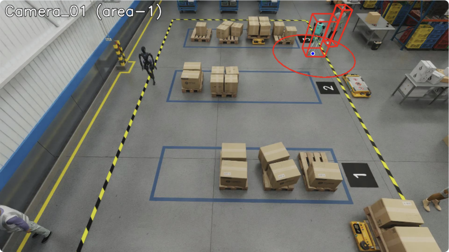
Proximity Violation

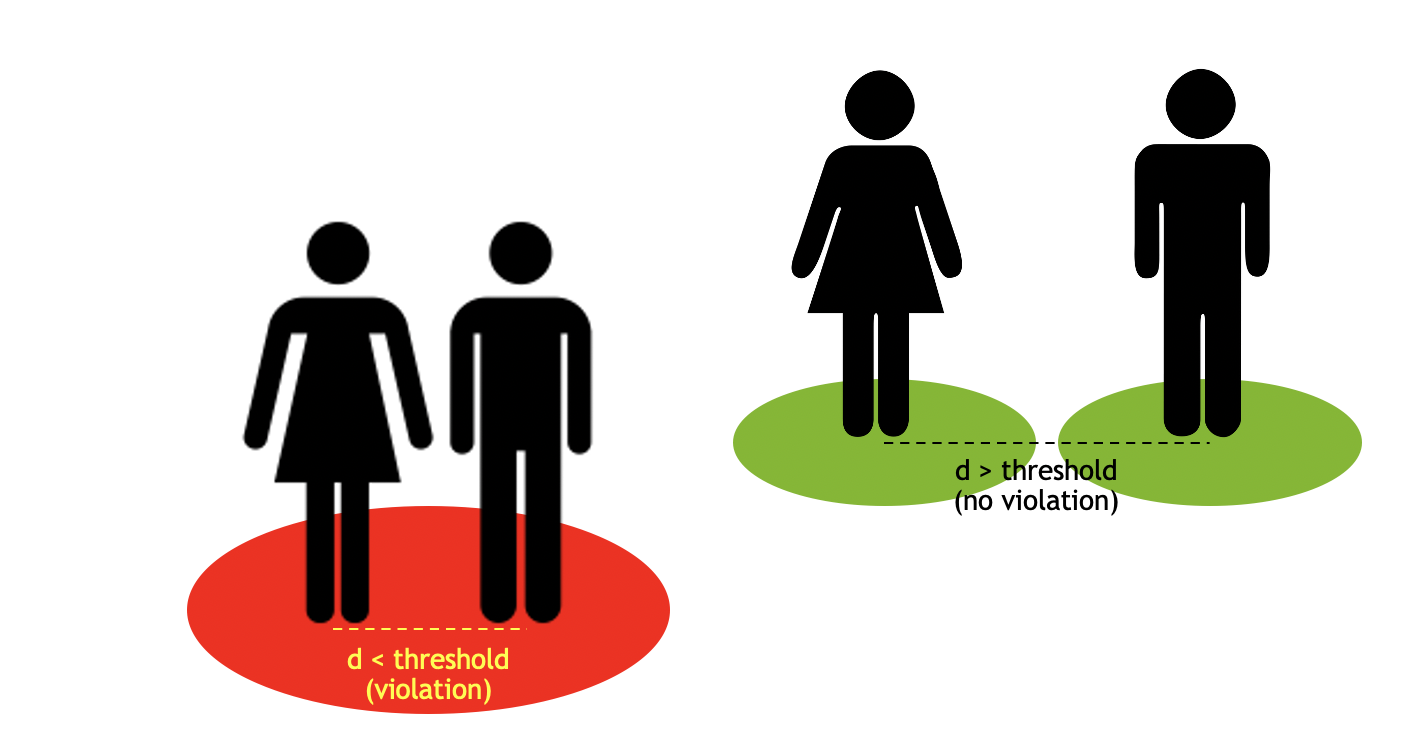
The objects detected are clustered via distance calculation and reports the cluster of points/objectIds involved in the violation.

The image below shows a proximity violation between a humanoid and a person. The distance between the two objects is less than the proximity threshold.

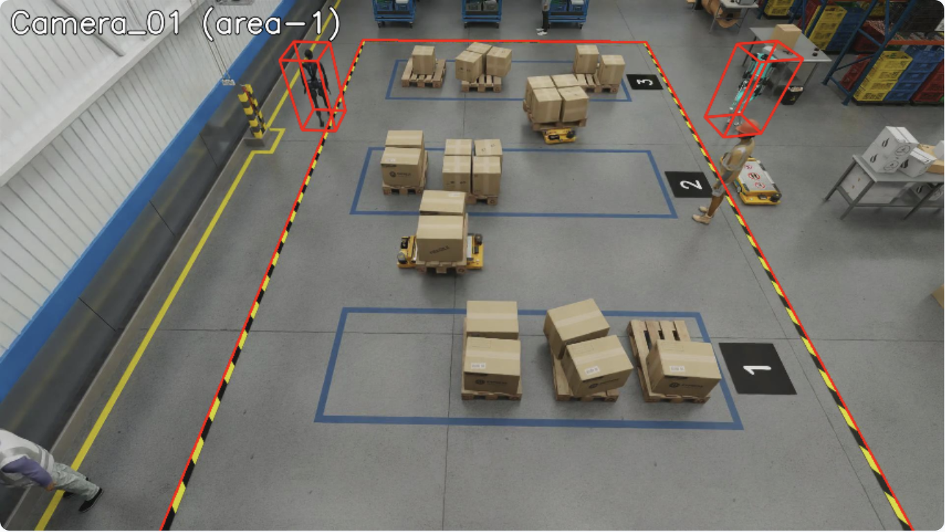
Confined Area Violation

The confined area violation is detected via point-in-polygon calculation. The system detects if any object is outside their designated confined area.

The image below shows the confined area violation. There are two humanoids present outside their designated confined areas. confinedObjectTypes for the area is set to “Humanoid” object type.

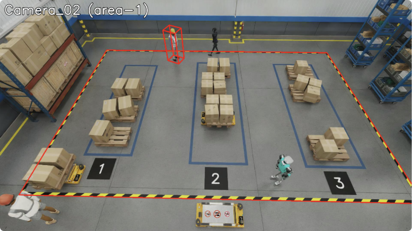
Restricted Area Violation

The restricted area violation is also detected via point-in-polygon calculation. The system detects if any object is inside their designated restricted area.

The image below shows the restricted area violation. One person is not allowed to be in the restricted area but is present inside it. restrictedObjectTypes for the same area is set to “Person” object type.

FOV Count Violation

The FOV count violation is triggered when the number of objects of a specific type in the field of view exceeds the configured threshold. This is useful for crowd control and capacity management scenarios.

The violation is configured via fovCountViolationIncidentObjectThreshold (maximum allowed count) and fovCountViolationIncidentObjectType (object type to count, e.g., “Person”).

Violation Detection API

from mdx.analytics.core.transform.calibration.calibration_e import CalibrationE
from mdx.analytics.core.transform.detection.proximity_detection import ProximityDetection

calibration = CalibrationE(app_config, calibration_file_path)
# Inside transform_frame:
# - Zone violations (restricted/confined) detected based on "restrictedObjectTypes" and "confinedObjectTypes"
# - FOV count computed per object type
enhanced_frames = [calibration.transform_frame(frame) for frame in batch_frames]

# Proximity violations detected separately via ProximityDetection
clusters, object_id_groups = ProximityDetection.cluster(center_objs, surrounding_objs, threshold)

Enhanced Frame Data

The transform_frame method generates FOV and ROI counts in the enhanced frame:

{
  "fov": [
    {"type": "Person", "count": 2},
    {"type": "Vehicle", "count": 3}
  ],
  "rois": [
    {"id": "roi-1", "type": "Person", "count": 2},
    {"id": "roi-2", "type": "Vehicle", "count": 3}
  ]
}

Incident Generation

Violations are tracked over time, and when they persist beyond the configured threshold, they become incidents.

Time Parameters

Each violation type has configurable timing parameters:

Timing Parameters

Parameter	Description
Expiration Window	Maximum gap between detections before creating a new violation state (0.5-2 sec typical)
Incident Threshold	Minimum duration for a violation to become a reportable incident (0.1-3 sec typical)

Configuration

{
  "app": [
    {"name": "incidentObjectTtl", "value": "3600"},
    {"name": "proximityViolationIncidentEnable", "value": "true"},
    {"name": "proximityViolationIncidentThreshold", "value": "1"},
    {"name": "proximityViolationIncidentExpirationWindow", "value": "1"},
    {"name": "restrictedAreaViolationIncidentEnable", "value": "true"},
    {"name": "restrictedAreaViolationIncidentThreshold", "value": "1"},
    {"name": "restrictedAreaViolationIncidentExpirationWindow", "value": "1"},
    {"name": "confinedAreaViolationIncidentEnable", "value": "true"},
    {"name": "confinedAreaViolationIncidentThreshold", "value": "1"},
    {"name": "confinedAreaViolationIncidentExpirationWindow", "value": "1"},
    {"name": "fovCountViolationIncidentEnable", "value": "true"},
    {"name": "fovCountViolationIncidentObjectThreshold", "value": "1"},
    {"name": "fovCountViolationIncidentThreshold", "value": "1"},
    {"name": "fovCountViolationIncidentExpirationWindow", "value": "1"},
    {"name": "fovCountViolationIncidentObjectType", "value": "Person"}
  ]
}

Incident Configuration Parameters

Incident Parameters

Parameter	Description
incidentObjectTtl	TTL (time-to-live) in seconds for object presence data. Objects with no data within the TTL window will be cleaned up. Default: 3600
proximityViolationIncidentEnable	Enable proximity violation incident detection. Default: false
proximityViolationIncidentThreshold	Minimum duration (seconds) for proximity violation to become an incident. Default: 1
proximityViolationIncidentExpirationWindow	Maximum gap (seconds) between detections before creating new violation state. Default: 1
restrictedAreaViolationIncidentEnable	Enable restricted area violation incident detection. Default: false
restrictedAreaViolationIncidentThreshold	Minimum duration (seconds) for restricted area violation to become an incident. Default: 1
restrictedAreaViolationIncidentExpirationWindow	Maximum gap (seconds) between detections before creating new violation state. Default: 1
confinedAreaViolationIncidentEnable	Enable confined area violation incident detection. Default: false
confinedAreaViolationIncidentThreshold	Minimum duration (seconds) for confined area violation to become an incident. Default: 1
confinedAreaViolationIncidentExpirationWindow	Maximum gap (seconds) between detections before creating new violation state. Default: 1
fovCountViolationIncidentEnable	Enable FOV count violation incident detection. Default: false
fovCountViolationIncidentObjectThreshold	Maximum number of objects allowed in FOV before triggering violation. Default: 1
fovCountViolationIncidentThreshold	Minimum duration (seconds) for FOV count violation to become an incident. Default: 1
fovCountViolationIncidentExpirationWindow	Maximum gap (seconds) between detections before creating new violation state. Default: 1
fovCountViolationIncidentObjectType	Object type to count for FOV violations. Default: Person

Usage

from mdx.analytics.core.stream.state.frame.frame_state_management import FrameStateMgmt

# Initialize (within BaseApp context)
frame_manager = FrameStateMgmt(self.config)

# Enhanced frames from calibration.transform_frame()
enhanced_frames = [self.calibration.transform_frame(f) for f in frames]

# Update with enhanced frames containing violation data
frame_manager.update_frames("sensor_001", enhanced_frames)

# Get all incidents
incidents = frame_manager.get_incidents("sensor_001")

# Get specific incident types
proximity_incidents = frame_manager.get_proximity_violation_incidents("sensor_001")
restricted_incidents = frame_manager.get_restricted_area_violation_incidents("sensor_001")
confined_incidents = frame_manager.get_confined_area_violation_incidents("sensor_001")
fov_count_incidents = frame_manager.get_fov_count_violation_incidents("sensor_001")

Incident Structure

For object-specific violations (Proximity, Restricted Area, Confined Area):

Incident(
    timestamp=datetime,              # Start time
    end=datetime,                    # End time
    sensorId="sensor_001",           # Sensor ID
    objectIds=["obj1", "obj2"],      # Objects involved
    category="Proximity Violation",  # Incident type
    place=Place(name="Location"),    # Location name
    info={
        "primaryObjectId": "obj1",   # Primary object (for object-specific violations)
        "roiId": "zone_1",           # ROI ID (for area violations)
        "isComplete": "true"         # Present for completed violations
    }
)

When object presence is tracked (e.g. Proximity Violation, FOV Count Violation), info may also include objectTimeline: a JSON string mapping object IDs to lists of {start, end} intervals (ISO 8601) during the violation window.

FOV Count Violation incidents use a single state per sensor (no primary object). objectIds lists all objects that contributed to the violation; info has no primaryObjectId and may include objectTimeline. Call get_incidents() regularly so completed states are cleared and memory stays bounded.

Data Flow

Raw Frames (objects) → Frame Enhancement (calculates violations) →
Enhanced Frames → FrameStateMgmt.update_frames():
  1. Filter frames by time
  2. Complete expired violations (gap > expiration_window)
  3. Update violation states from frame fields
→ get_incidents():
  1. Generate incidents from active states (duration >= threshold)
  2. Generate incidents from completed states
  3. Clear processed completed states

Sink

The pipeline supports multiple sink types for publishing processed data:

• Kafka Sink: Publishes data to Kafka topics.

• Redis Streams Sink: Publishes data to Redis Streams for lightweight deployments.

• MQTT Sink: Publishes data to MQTT topics for IoT-oriented deployments.

The sink type is configured via the sinkType parameter in the app configuration section. Set it to kafka, redisStream, or mqtt based on your deployment requirements.

Usage with BaseApp

When using BaseApp, the sink is automatically initialized and available via built-in write methods:

from mdx.analytics.core.app.app_base import BaseApp
from mdx.analytics.core.utils.processing_stats import BatchStats

class MyApp(BaseApp):
    def process(self, frames, stats: BatchStats):
        # Write enhanced frames
        enhanced = [self.calibration.transform_frame(f) for f in frames]
        self.write_frames(enhanced)

        # Write behaviors
        self.write_behaviors(behaviors)

        # Write events (tripwire, ROI)
        self.write_events(events)

        # Write incidents from violation detection
        self.write_incidents(incidents)

        # Write anomalies
        self.write_anomalies(anomalies)

        # Write behaviors with trajectory clustering
        self.write_behaviors_with_clustering(behaviors)

        # Write space utilization data
        self.write_space_utilization(space_utilization_data)

Standalone Sink Usage

For standalone usage without BaseApp, use the sink factory:

from mdx.analytics.core.stream.sink.sink_factory import get_sink
from mdx.analytics.core.stream.sink.sink_base import ProtoBytesSerializer, StrBytesSerializer
from mdx.analytics.core.schema.config import AppConfig

config = AppConfig(**config_data)
sink = get_sink(config)  # Returns SinkKafka, SinkRedisStream, or SinkMQTT

# Write protobuf messages to a destination
sink.write(
    dest_key="behavior",
    messages=behavior_protos,
    value_serializer=ProtoBytesSerializer,
    key_extractor=lambda b: b.sensor.id,
    key_serializer=StrBytesSerializer
)

# Close when done
sink.close()

API

BaseApp write methods (recommended):

class BaseApp:
    # Write enhanced frames to the frames topic
    def write_frames(self, frames: list[nvSchema.Frame]) -> None

    # Write behaviors to the behavior topic
    def write_behaviors(self, behaviors: list[Behavior]) -> None

    # Write events to the events topic
    def write_events(self, events: list[Behavior]) -> None

    # Write incidents to the incidents topic
    def write_incidents(self, incidents: list[Incident]) -> None

    # Write anomalies to the anomaly topic
    def write_anomalies(self, anomalies: list[Behavior]) -> None

    # Write space utilization data
    def write_space_utilization(self, output: list[SpaceUtilization]) -> None

    # Write behaviors with clustering to behaviorPlus topic
    def write_behaviors_with_clustering(self, behaviors: list[Behavior]) -> None

Low-level Sink interface:

class Sink:
    # Write messages to a destination with serialization
    def write(
        self,
        dest_key: str,                      # Destination stream key
        messages: list[Any],                # Messages to write
        value_serializer: Callable,         # Serialize message values
        key_extractor: Callable | None,     # Extract keys from messages
        key_serializer: Callable | None,    # Serialize message keys
        headers: Mapping[str, bytes] | None # Optional headers
    ) -> None

    # Write a single message
    def write_msg(
        self,
        dest_key: str,
        message: bytes,
        key: bytes | None,
        headers: Mapping[str, bytes] | None
    ) -> None

    # Close the sink
    def close(self) -> None

Note

You can develop custom sink implementations by extending the Sink base class.

Customization in your deployment

You can customize code by extracting a file from the Behavior Analytics Docker image, editing it on your host, and mounting it into the container via Docker Compose. The container uses the mounted file instead of the one baked into the image. All code of the installed analytics library is under /usr/local/lib/python3.13/site-packages/mdx/analytics/core.

General pattern

1. Get the file from the image — Run the image and print the file contents (or copy it out), then save to a file on your host.

2. Edit the file — Apply your code changes locally.

3. Mount and run — In your Compose file (e.g. warehouse-2d-app.yml), add a volume mapping from your host file to the path inside the container under /usr/local/lib/python3.13/site-packages/mdx/analytics/core/.... Restart the stack.

Step 1: Get the file from the image

The image is distroless (no shell). Run the image with python3 -c "..." to print the file contents. Replace <path/to/module.py> with the path to the module file under .../site-packages/mdx/analytics/core/ (e.g. transform/calibration/my_module.py). Save the output to a file on your host:

docker run --rm <behavior-analytics-image> \
  python3 -c "print(open('/usr/local/lib/python3.13/site-packages/mdx/analytics/core/<path/to/module.py>').read())"

Redirect the output to a file (e.g. > module.py), or copy-paste into your editor and save.

Step 2: Change the file

Edit the file as needed on your host.

Step 3: Mount and run

In your deployment YAML file (e.g. warehouse-2d-app.yml), under the volumes: section for the analytics service, add:

- path/to/your/module.py:/usr/local/lib/python3.13/site-packages/mdx/analytics/core/<path/to/module.py>

Replace path/to/your/module.py with your host path and <path/to/module.py> with the same path used in Step 1. Restart the deployment.

Dynamic Calibration

The system supports dynamic calibration at runtime. BaseApp uses the DynamicCalibration wrapper which:

1. Type detection: Reads calibrationType (image, cartesian, geo) from JSON; missing/unknown → image (CalibrationI).

2. No file at startup: Starts with image; a file can be added later for a one-time switch to cartesian or geo.

3. File monitoring: Watches the calibration directory; if started with a file, changes only reload data (type does not switch).

4. Notification listener: Listens to mdx-notification.

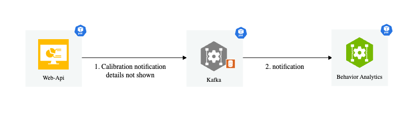
How It Works

When BaseApp starts:

1. DynamicCalibration is initialized with the optional calibration file path

2. calibration.start_listen() is called to start file monitoring

3. CalibrationListener is started by AppRunner to listen for notifications

4. When a notification is received, it writes the new calibration to a file

5. The file monitor detects the change and reloads the calibration data

Notification Message Format

 "topic": "mdx-notification"
 "key": "calibration"

 "value": {
  "version": "1.0",
  "calibrationType": "cartesian",
  "sensors": [
     "...sensor definitions..."
  ]
 }

"headers": {
 "event.type": "upsert or upsert-all or delete",
 "timestamp": "2021-06-01T14:34:13.417Z"
}

Usage with BaseApp

When using BaseApp, dynamic calibration is handled automatically:

from mdx.analytics.core.app.app_base import BaseApp
from mdx.analytics.core.app.app_runner import run

class MyApp(BaseApp):
    def __init__(self, config, calibration_path):
        super().__init__(config, calibration_path)
        # self.calibration is DynamicCalibration, automatically initialized
        # File monitoring is started automatically

if __name__ == '__main__':
    run(MyApp)  # AppRunner starts CalibrationListener automatically

Standalone Usage

For standalone usage:

from mdx.analytics.core.transform.calibration.calibration_dynamic import DynamicCalibration
from mdx.analytics.core.transform.calibration.calibration_listener import CalibrationListener
from mdx.analytics.core.stream.source.source_factory import get_source

# Initialize dynamic calibration
calibration = DynamicCalibration(config, calibration_path)
calibration.start_listen()  # Start file monitoring

# Set up notification listener
source = get_source(config)
listener = CalibrationListener(config, read_notifications_func)
listener.start()

API

class DynamicCalibration:
    # Initialize with automatic type detection
    def __init__(self, config: AppConfig, calibration_path: str | None) -> None

    # Start file monitoring for calibration changes
    def start_listen(self) -> None

    # Get the current calibration type
    @property
    def calibration_type(self) -> CalibrationType

    # All CalibrationBase methods are available via delegation
    def transform(self, msg: Message) -> Message
    def transform_frame(self, frame: nvSchema.Frame) -> nvSchema.Frame
    def filter_frames_by_sensor_id(self, frames: list[nvSchema.Frame]) -> list[nvSchema.Frame]

class CalibrationListener:
    # Initialize with config and notification reader function
    def __init__(self, config: AppConfig, read_notifications: Callable) -> None

    # Start listening for notifications
    def start(self) -> None

    # Stop listening
    def close(self) -> None

Space Utilization

Space utilization is a feature that allows you to analyze the space occupied by objects in a given area. It can be used to monitor the utilization of a warehouse, parking lot, or any other space where objects are present. It is initially designed for monitoring the utilization of the buffer zones in a warehouse, but can be extended to other use cases as well.

Usage

Initialize the SpaceAnalyzer with the app config and calibration file, then invoke the analyze method to analyze space utilization in specified zones, calculating metrics such as occupied space, free space, and maximum additional pallets that can be placed. It supports both genetic algorithm and greedy search approaches for pallet placement optimization.

The details on the designated config parameters can be found in the above space analytics config section.

from mdx.analytics.core.utils.space_utilization import SpaceAnalyzer

space_analyzer = SpaceAnalyzer(app_config.spaceAnalytics, calibration)
outputs_nv, outputs_dict = space_analyzer.analyze(messages_map, pallet_width=1.0, target_zones=["zone1"])

Output

The main methods analyze returns the computed space utilization metrics in two formats:

1. NV schema format: This is the default output format, which is used in the space utilization app.

2. Dictionary format: This is a more general output format used by agents, which includes additional information such as the objects bounding boxes for visualization uses.

Below we list out the key metrics along with the brief description that are included in the output.

Space Utilization Metrics

Name	Description
spaceOccupied	area size of the occupied space (in square meters)
freeSpace	area size of the free space (in square meters)
totalSpace	area size of the total space (in square meters)
spaceUtilization	the ratio/percentage that the total space is utilized/occupied
numExtraPallets	the max number of extra pallets that can fit into the free space
utilizableFreeSpace	area size of the utilizable free space
freeSpaceQuality	the ratio/percentage that the free space is utilizable
isUnsafe	flag to indicate if unsafe conditions exist (pallets placed outside buffer zone boundaries)
unsafePalletCnt	count of pallets flagged as unsafe (placed partially outside the buffer zone beyond the unsafeSize threshold)

The layouts of the free space and utilizable free space are also included in the output. NV schema output format follows exactly the definition in JSON Schema, please refer to JSON Schema for more details.

The dictionary format output also includes the bounding boxes of the objects in the scene for visualization purposes. The dictionary format output is consumed directly in agent workflows. Below is a sample output of the dictionary format:

[
  {
      "id": "buffer_zone_1",
      "timestamp": "2025-02-10 17:53:47.002000+00:00",
      "metrics": {
          "spaceOccupied": 1.73,
          "freeSpace": 8.65,
          "totalSpace": 10.38,
          "spaceUtilization": 0.17,
          "numExtraPallets": 2,
          "utilizableFreeSpace": 2.0,
          "freeSpaceQuality": 0.23,
          "isUnsafe": false,
          "unsafePalletCnt": 0
      },
      "sensors": [],
      "layouts": {
          "freeSpace": [
              [
                  [
                      [
                          4.536781311035156,
                          -11.159529685974121
                      ],
                      "..."
                  ]
              ]
          ],
          "utilizableFreeSpace": [
              [
                  [
                      [
                          6.389277935028077,
                          -12.959529685974122
                      ],
                      "..."
                  ]
              ],
              "..."
          ]
      },
      "bboxes": {
          "occupiedObj": [
              [
                  6.01904,
                  -12.389612,
                  0.468785,
                  0.554186,
                  0.731014,
                  0.521152,
                  0.0,
                  0.0,
                  1.635653
              ],
              "..."
          ],
          "unsafeObj": []
      }
  },
  "..."
]

Logic and Method

The logic to compute the space utilization metrics is described as follows:

• Everything is projected from 3D to 2D floor space (top-down view) of the moniored area.

• totalSpace is the size of the designated buffer zone which is on the floor plane.

• spaceOccupied is the total area within the buffer zone that is occupied by target objects. Typical target objects are pallets and boxes. The detected 3D bounding boxes of the target objects are projected onto the floor plane and total size of the projected area (within the buffer zone) is calculated.

• freeSpace is calculated as totalSpace - spaceOccupied.

• spaceUtilization is calculated as spaceOccupied / totalSpace.

• numExtraPallets is calculated as the maximum number of extra pallets that can fit into the free space.

• utilizableFreeSpace is calculated as numExtraPallets * pallet size.

• freeSpaceQuality is calculated as utilizableFreeSpace / freeSpace.

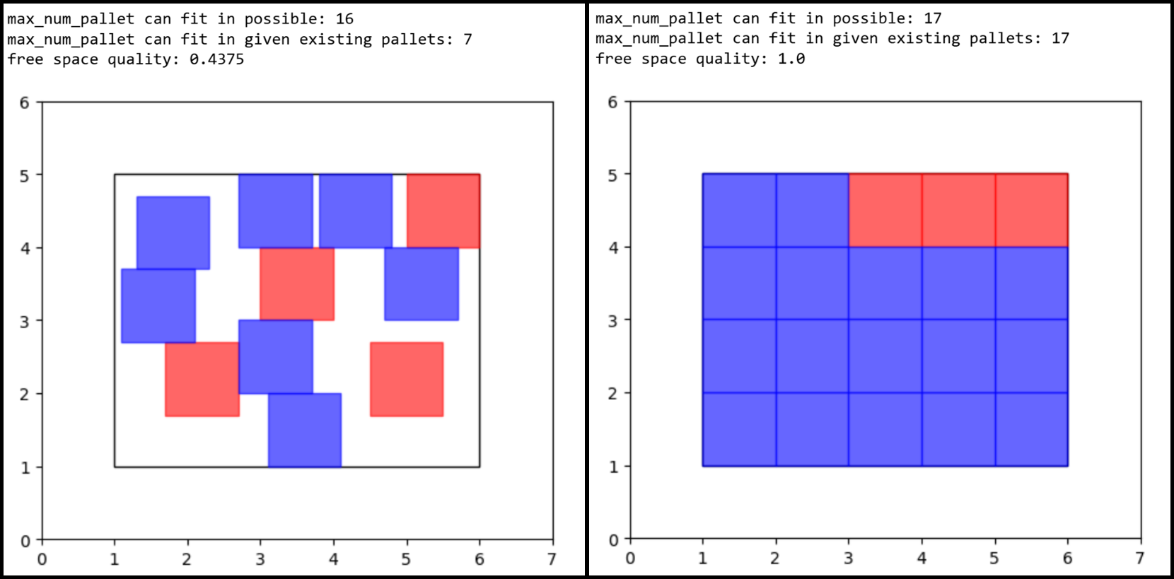
The computation of freeSpaceQuality is demonstrated in the figure below. The black rectangle indicates a 4-by-5 buffer zone, the spares are pallets with size 1-by-1, red squares are existing pallets in the buffer zone and blue squares are the extra pallets that can still be placed in, assuming all units are in meters. In the right case the 3 existing pallets are placed tightly together in a corner and the free space can be fully utilized to place 17 extra pallets thus the freeSpaceQuality is 100%. In the left case the 4 existing pallets are placed spreading out thus only 7 extra pallets can be placed in the free space which yields 43.75% as the freeSpaceQuality.

The key value and trickiest one to compute here is numExtraPallets. Finding the maximum number extra of pallets is an optimization problem to find the best placement strategy to fit the most pallets into the free space under the condition that pallets cannot be overlapping with each other or with existing objects in the buffer zone. To find this optimal placement strategy we provide two different search algorithms as options here: genetic algorithm (GA) and greedy search.

• Genetic algorithm logic is constructed as follows:

  • Genome = the placement plan of N pallets: [(x1,y1), (x2,y2), …., (xN,yN)] there (x,y) is the center location of each pallet.

  • Fitness score = the negative value of number of crosses between the N pallets and against the buffer zone boundaries + the existing pallets. So here fitness score is <=0, the larger the better, if fitness score=0 reached which means a placement plan is found, in other words: N pallets can be fit in the free area.

  • Crossover is randomly swap two genomes (x1,y1) and (x2,y2) to (x1,y2) and (x2,y1)

  • Mutation is randomly add delta to (x1,y1) and (x2,y2) to (x1+delta,y1+delta) and (x2+delta,y2+delta)

  • We gradually increase N and find the largest N with fitness score=0, which is the maximum number of pallets that can fit in the free space.

• Greedy search logic is constructed as follows:

  • Place extra pallets one at a time util no more pallets can be fit in.

  • Try to put a pallet in the top-left corner of the buffer zone.

  • If it fits in, Tty to put a new pallet in, starting from the initial location next to the previous one

  • If it doesn’t fit in, slide it X distance to the right and try again (if reach right end, slide down and start from the very left)

  • If no more pallets can be fit in, stop and return the number of pallets that have been fit in.

Under the simplified assumption of rectangle-shaped buffer zone and square-shaped pallet of our current use case, Greedy Search provides on-par or better accuracy and much faster processing speed comparing to GA. Greedy search is the default method used in the space utilization app, and user can also choose to use GA by setting the useGA parameter to true in the space analytics config section.

Other Tools

Under py-analytics-stream library, we created tools for warehouse blueprint agents to use in various agentic workflows.

Space Utilization Tool

API

The class and key method definitions for the Space Utilization tool are as follows:

class SpaceUtilization(config_path: str, calibration_path: str = None)

Controller module for Space Utilization Analytics.

Parameters:

• config_path (str) – Path to the app config file.

• calibration_path (Optional[str]) – Path to the calibration file in JSON format. If not provided, calibration will be initialized from API.

Variables:

• config (AppConfig) – Application configuration object.

• calibration (CalibrationE) – Calibration module for coordinate transformation.

• space_analyzer (SpaceAnalyzer) – Space analysis module.

• cam_font_size (float) – Font size for camera annotations.

• in_3d_mode (bool) – Whether to use 3D mode for visualization.

space_analysis_on_demand(

detections: str,

pallet_width: float = 1.0,

target_zones: List[str] = [],

frames_from_file: bool = False,

) → List[Dict[str, Any]]

Analyze space utilization from detection data.

This method: 1. Loads detection data from file or uses provided data 2. Converts detection data to protobuf format 3. Processes detections through space analyzer 4. Returns analysis results for specified zones

Parameters:

• detections (str) – Detection data or path to JSON file containing detection data.

• pallet_width (float) – Width of pallets in meters. Defaults to 1.0.

• target_zones (List[str]) – List of zone IDs to analyze. If empty, analyzes all zones.

• frames_from_file (bool) – Whether detections parameter is a file path. Defaults to False.

Returns:

List of dictionaries containing analysis results for each zone.

Return type:

List[Dict[str, Any]]

Example:

>>> space_utilization_tool = SpaceUtilization(
...     config_path="config.json",
...     calibration_path="calibration.json"
... )
>>> outputs = space_utilization_tool.space_analysis_on_demand(
...     detections="detections.json",
...     pallet_width=1.0,
...     target_zones=["zone1", "zone2"],
...     frames_from_file=True
... )

projection_3d_on_demand(

outputs_dict: List[Dict[str, Any]],

image_path: str,

sensor_id: str,

output_size: Tuple[int, int] = (960, 540),

show_unsafe_pallets: bool = True,

export_base64: bool = True,

font_size: float | None = None,

title: str | None = None,

) → str | np.ndarray

Project 3D analysis results onto a 2D image.

This method: 1. Loads base image from file 2. For each analyzed zone:

• Overlays unsafe pallets or free space visualization

• Applies annotations and titles

3. Resizes output to specified dimensions

4. Optionally converts to base64 string

Parameters:

• outputs_dict (List[Dict[str, Any]]) – Analysis results from space_analysis_on_demand.

• image_path (str) – Path to the image file to overlay results on.

• sensor_id (str) – ID of the camera sensor.

• output_size (Tuple[int, int]) – Output image dimensions (width, height). Defaults to (960, 540).

• show_unsafe_pallets (bool) – Whether to show unsafe pallets. Defaults to True.

• export_base64 (bool) – Whether to return image as base64 string. Defaults to True.

• font_size (Optional[float]) – Font size for annotations. If None, uses default from config.

• title (Optional[str]) – Title to display on image. If None, uses sensor_id.

Returns:

Base64 encoded image string if export_base64=True, otherwise numpy array.

Return type:

Union[str, np.ndarray]

Example:

>>> space_utilization_tool = SpaceUtilization(
...     config_path="config.json",
...     calibration_path="calibration.json"
... )
>>> image = space_utilization_tool.projection_3d_on_demand(
...     outputs_dict=analysis_results,
...     image_path="camera1.jpg",
...     sensor_id="Camera_01",
...     show_unsafe_pallets=True
... )

viz_frame_alerts(

mdx_frame_alerts: str | Dict[str, Any],

image_path: str,

sensor_id: str,

output_size: Tuple[int, int] = (960, 540),

frames_from_file: bool = False,

export_base64: bool = False,

title: str | None = None,

font_size: float | None = None,

) → str | np.ndarray

Visualize frame alerts including proximity, confined area, and restricted area alerts.

This method:

1. Reads and processes frame alerts data

2. Applies visualization for different alert types:

   • Proximity alerts between objects

   • Confined area violations

   • Restricted area violations

3. Applies color and thickness settings from config

4. Adds title and annotations

5. Resizes and optionally exports as base64

Parameters:

• mdx_frame_alerts (Union[str, Dict[str, Any]]) – Frame alerts data or path to JSON file.

• image_path (str) – Path to the image file to overlay alerts on.

• sensor_id (str) – ID of the camera sensor.

• output_size (Tuple[int, int]) – Output image dimensions (width, height). Defaults to (960, 540).

• frames_from_file (bool) – Whether mdx_frame_alerts is a file path. Defaults to False.

• export_base64 (bool) – Whether to return image as base64 string. Defaults to False.

• title (Optional[str]) – Title to display on image. If None, uses sensor_id.

• font_size (Optional[float]) – Font size for annotations. If None, uses default from config.

Returns:

Base64 encoded image string if export_base64=True, otherwise numpy array.

Return type:

Union[str, np.ndarray]

Example:

>>> space_utilization_tool = SpaceUtilization(
...     config_path="config.json",
...     calibration_path="calibration.json"
... )
>>> image = space_utilization_tool.viz_frame_alerts(
...     mdx_frame_alerts="alerts.json",
...     image_path="camera1.jpg",
...     sensor_id="Camera_01",
...     frames_from_file=True
... )

Config

The full config file for the SpaceUtilization tool is shown below:

{
  "app": [
    {
      "name": "in3dMode",
      "value": "true"
    },
    {
      "name": "apiMDX",
      "value": "http://10.117.4.39:8081"
    },
    {
      "name": "apiRetryMaxCnt",
      "value": "5"
    },
    {
      "name": "apiRetryMaxTimeSec",
      "value": "5"
    },
    {
      "name": "cameraFontSize",
      "value": "2"
    },
    {
      "name": "advancedOverlay",
      "value": "false"
    },
    {
      "name": "spaceAnalyticsIntervalSec",
      "value": "1.0"
    },
    {
      "name": "spaceAnalyticsGridSize",
      "value": "0.2"
    },
    {
      "name": "spaceAnalyticsUnsafeSize",
      "value": "0.5"
    },
    {
      "name": "spaceAnalyticsTargetClasses",
      "value": "[\"Box\", \"Pallet\", \"Transporter\", \"Crate\"]"
    },
    {
      "name": "spaceAnalyticsUseGA",
      "value": "false"
    },
    {
      "name": "spaceAnalyticsPopulationSizeGA",
      "value": "100"
    },
    {
      "name": "spaceAnalyticsNumGenerationsGA",
      "value": "100"
    },
    {
      "name": "confinedBboxColorRGB",
      "value": "255, 128, 0"
    },
    {
      "name": "confinedROIColorRGB",
      "value": "255, 128, 0"
    },
    {
      "name": "confinedBboxThickness",
      "value": "3"
    },
    {
      "name": "confinedROIThickness",
      "value": "4"
    },
    {
      "name": "restrictedBboxColorRGB",
      "value": "153, 0, 0"
    },
    {
      "name": "restrictedROIColorRGB",
      "value": "153, 0, 0"
    },
    {
      "name": "restrictedBboxThickness",
      "value": "3"
    },
    {
      "name": "restrictedROIThickness",
      "value": "2"
    },
    {
      "name": "proximityCenterObjType",
      "value": "Agility_Digit_Humanoid"
    },
    {
      "name": "proximityThickness",
      "value": "3"
    }
  ]
}

Space analytics parameters (spaceAnalyticsIntervalSec, spaceAnalyticsGridSize, etc.) follow the same naming convention as described in the space analytics config section. The extra parameters in the app section are described below:

Space Utilization Tool Config Parameters

Name	Default	Description
in3dMode	false	Whether to use 3D mode for visualization. If set to true, the tool will use 3D projection for visualization.
apiMDX	http://localhost:8081	URL of the MDX API for fetching calibration and asset.
apiRetryMaxCnt	30	Maximum number of retries for API calls of fetching calibration / asset. If maximum is reached for fetching calibration, space utilization tool initialization will fail.
apiRetryMaxTimeSec	30	Maximum time in seconds to wait for API response of fetching calibration / asset. If maximum is reached for fetching calibration, space utilization tool initialization will fail.
cameraFontSize	2	Font size for camera annotations.
advancedOverlay	true	Whether to use advanced overlay for visualization.
confinedBboxColorRGB	255, 128, 0	RGB color for bounding box of confined area violation objects.
confinedROIColorRGB	255, 128, 0	RGB color for confined area ROI.
confinedBboxThickness	3	Thickness of bounding box lines of confined area violation objects.
confinedROIThickness	4	Thickness of confined area ROI lines.
restrictedBboxColorRGB	153, 0, 0	RGB color for bounding box of restricted area violation objects.
restrictedROIColorRGB	153, 0, 0	RGB color for restricted area ROI.
restrictedBboxThickness	3	Thickness of bounding box lines of restricted area violation objects.
restrictedROIThickness	2	Thickness of restricted area ROI lines.
proximityCenterObjType	Humanoid	Object type used as the center for proximity detection.
proximityThickness	3	Thickness of proximity detection lines.

Samples

Sample space utilization visualization is shown below. The green color patch indicates the extra pallets that can be placed in the free space, and the blue color shows the rest of the free space.

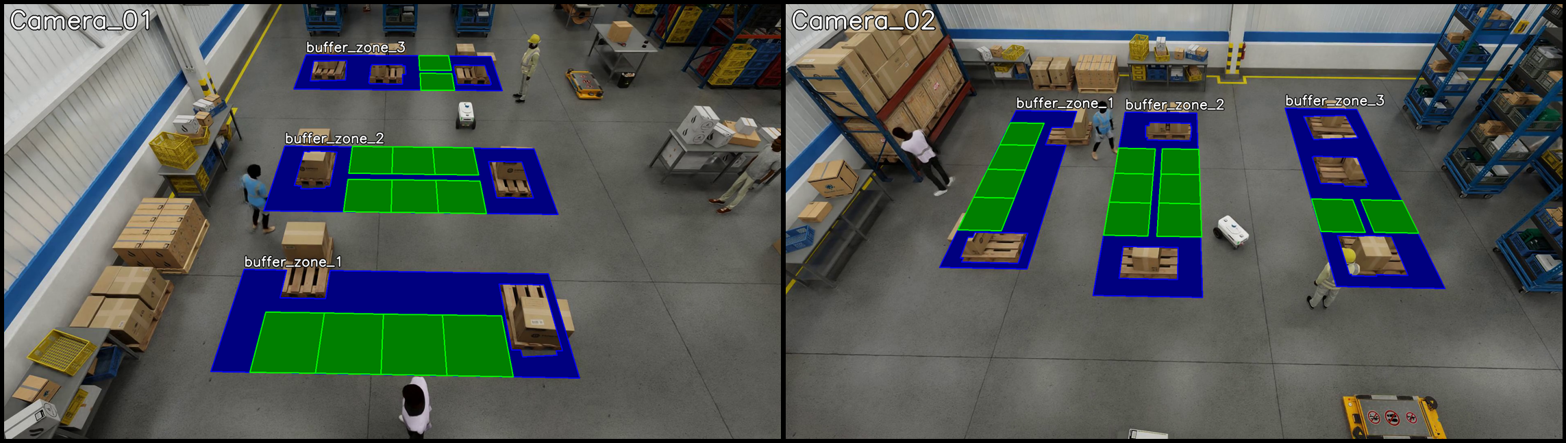
When visualizing space utilization, if advancedOverlay is set to true, the tool will make the color patch transparent as well as avoid overlapping on the existing objects (boxes/pallets) in the buffer zone. This makes image visualization more intuitive to read but will also introduce extra computation time. For reference, a single visualization invocation time goes from 0.04sec to 1.7sec when using advanced overlay. Sample space utilization visualization with advanced overlay is shown below.

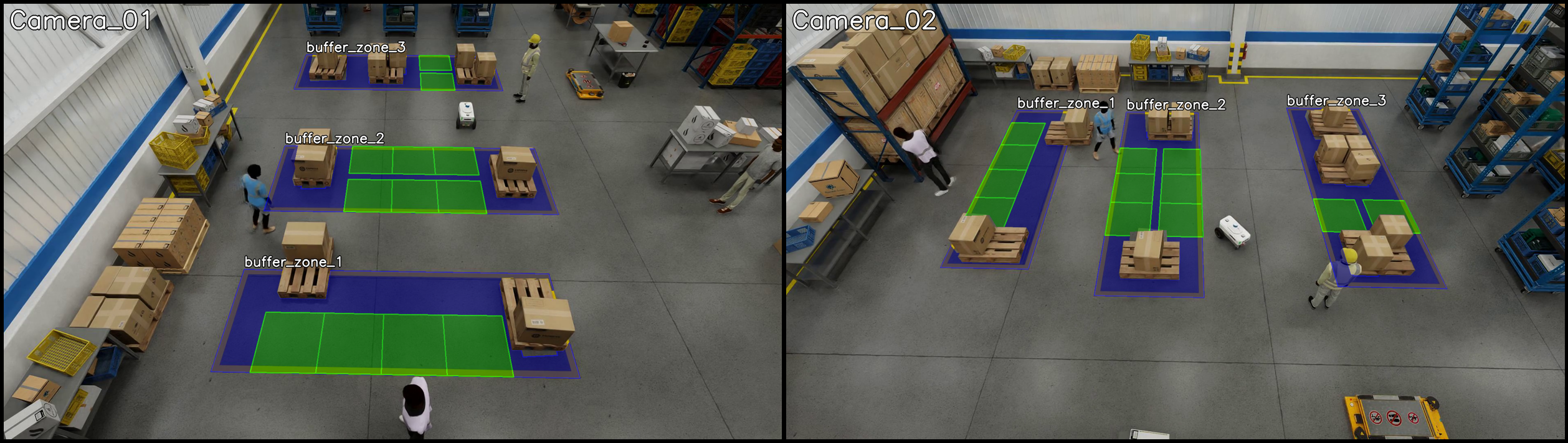
Sample visualizations of frame alerts are shown below. The dark red color bounding box highlights the restricted area violation objects. The orange color bounding box shows the confined area violation objects. The blue color bounding box shows the center object of a proximity violation detection, the red circle indicates the proximity range and the red bounding box highlights the proximity violation object.

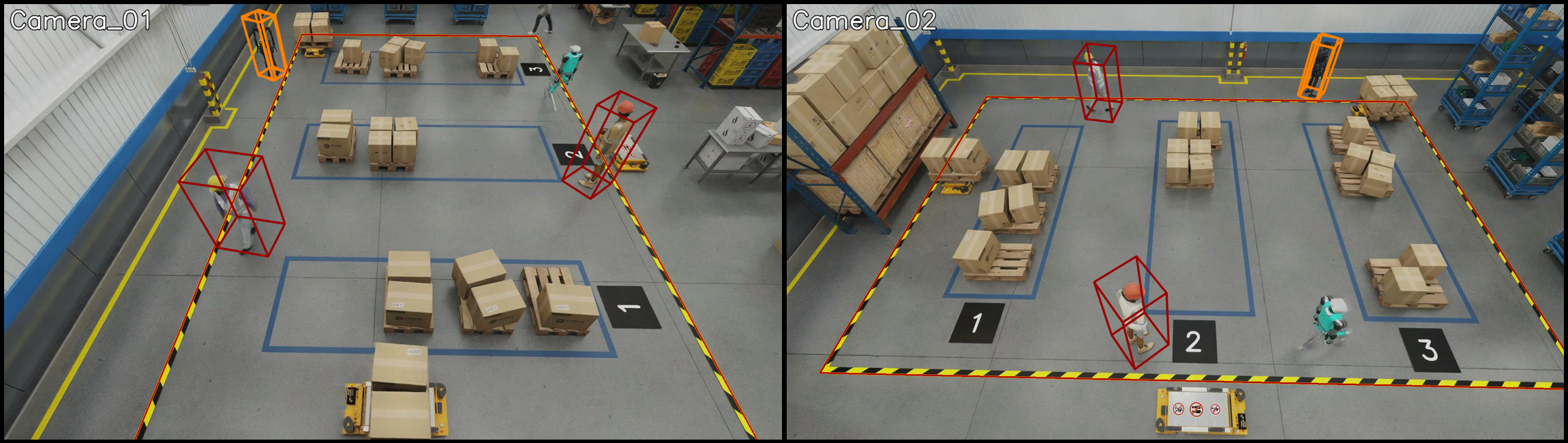
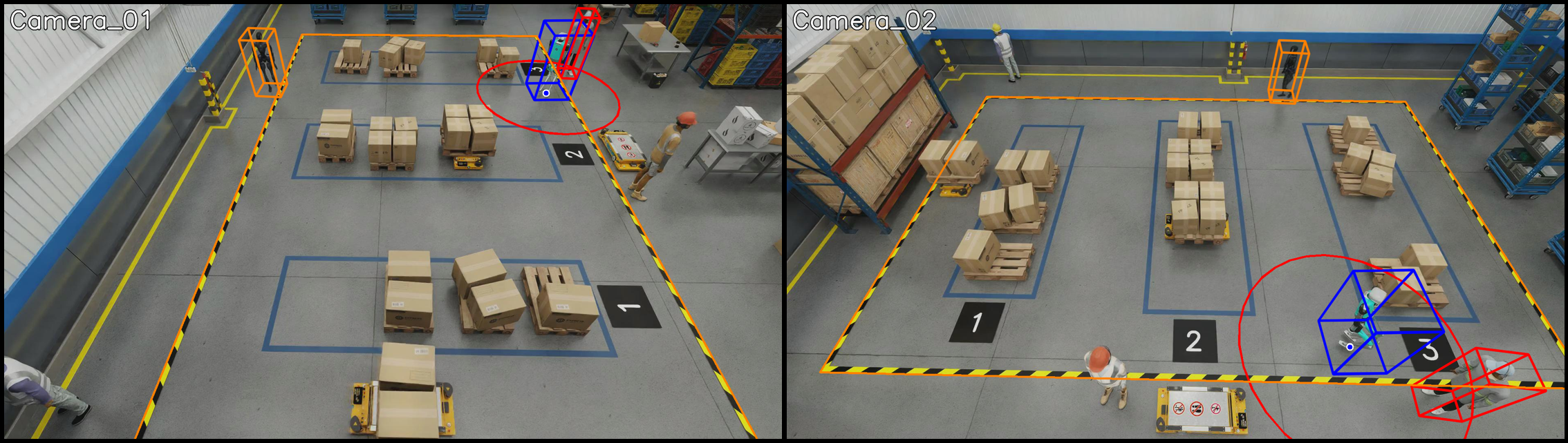
USD Search Tool

The USD Search tool is a module designed to provide the agent knowledge of the study environment. In our sample warehouse blueprint workflows, synthetic data is used and the study environment is the USD asset. USD Search tool has an option to use USD Search API as the endpoint to query the USD asset, and that is how we named it this way initially. Essentially the Asset Graph Service (AGS) API is the only part used from USD search APIs. The alternative to using AGS API is to use mdxAPI for fetching asset information. mdxAPI is required for the calibration anyways thus using it for asset information as well removing the dependency on AGS API.

USD Search tool is used for tasks such as:

• Finding the size of a specific object (e.g. pallet)

• Finding the dimension of a specific area (e.g. buffer zone)

• Finding the best camera to view a specific area

• Finding the best camera to view a set of specific objects

• Finding the id used within the system of sub-areas and groups

API

The class and key method definitions for the USD Search tool are as follows:

class USDSearch(

config_path: str,

calibration_path: str = None,

asset_json_path: str = None,

)

A controller module for searching and analyzing USD (Universal Scene Description) scene elements.

The class supports loading data either from JSON files or through API endpoints. Controlled by configuration settings.

Parameters:

• config_path (str) – Path to the app config file.

• calibration_path (Optional[str]) – Path to the calibration file in JSON format.

• asset_json_path (Optional[str]) – Path to the asset JSON file.

Variables:

• config (AppConfig) – Application configuration object.

• calibration (CalibrationE) – Calibration module for coordinate transformation.

• asset_dict (dict) – Dictionary containing asset information.

• prim_query_base_url (str) – Base URL for primitive queries.

• prim_pallets (list) – List of pallet primitives.

• prim_buffer_zones (list) – List of buffer zone primitives.

• prim_cameras (list) – List of camera primitives.

• pallet_size_map (dict) – Mapping of pallet IDs to their sizes.

• buffer_zone_to_camera_map (dict) – Mapping of buffer zones to cameras.

• bev_camera_map (dict) – Mapping of BEVs to cameras.

• camera_fov_coverage_map (dict) – Mapping of cameras to their FOV coverage.

get_pallet_size(pallet_id: str) → float | None

Get the size of a pallet given its ID.

This method:

1. Checks if pallet size map exists, fetches if not

2. Looks up the pallet ID in the size map

3. Returns the size or None if not found

The size is calculated as the square root of the pallet’s area (width * length).

Parameters:

pallet_id (str) – The ID of the pallet to look up.

Returns:

The size of the pallet, or None if not found.

Return type:

Optional[float]

Example:

>>> usd_search = USDSearch("config.json")
>>> size = usd_search.get_pallet_size("Pallet_A1")
>>> # Example output: 1.25

get_buffer_zone_dimensions(buffer_zone_id: str) → List[List[float]]

Get the dimensions of a buffer zone given its ID.

This method:

1. Retrieves available ROIs from calibration

2. Searches for the specified buffer zone

3. Returns coordinates if found, empty list if not

Parameters:

buffer_zone_id (str) – The ID of the buffer zone to look up.

Returns:

List of [x,y] coordinates defining the buffer zone dimensions, or empty list if not found.

Return type:

List[List[float]]

Example:

>>> usd_search = USDSearch("config.json")
>>> dimensions = usd_search.get_buffer_zone_dimensions("zone_1")
>>> # Example output: [[0.0, 0.0], [1.0, 0.0], [1.0, 1.0], [0.0, 1.0]]

get_best_camera_on_buffer_zones(

buffer_zones: list = [],

) → str | None

Get best camera for viewing multiple buffer zones.

This method:

1. Gets lists of cameras for each buffer zone

2. Finds cameras that can see all zones

3. Calculates combined score for each camera

4. Returns camera with highest score

The camera score is based on:

• Number of buffer zones visible

• Coverage area of each zone

• Balance of visibility across zones

Parameters:

buffer_zones (list) – List of buffer zone IDs. If empty, analyzes all buffer zones.

Returns:

ID of best camera for viewing all specified buffer zones, or None if not found.

Return type:

Optional[str]

Example:

>>> usd_search = USDSearch("config.json")
>>> # Get best camera for specific zones
>>> best_camera = usd_search.get_best_camera_on_buffer_zones(["zone_1", "zone_2"])
>>> # Get best camera for all zones
>>> best_camera_all = usd_search.get_best_camera_on_buffer_zones()

get_zone_camera_bev_on_areas(

areas: list = [],

) → Tuple[list, list, list, list]

Get mapping of areas to buffer zones, cameras and BEVs (Bird’s Eye Views).

This method:

1. Gets BEVs for specified areas

2. Gets buffer zones for each BEV

3. Gets best camera for each buffer zone group

4. Returns lists of zones, cameras, BEVs, and areas

Parameters:

areas (list) – List of area IDs. If empty, analyzes all areas.

Returns:

Tuple containing (buffer_zones_list, camera_list, bev_id_list, area_id_list).

Return type:

Tuple[List[List[str]], List[str], List[str], List[str]]

Example:

>>> usd_search = USDSearch("config.json")
>>> zones, cameras, bevs, areas = usd_search.get_zone_camera_bev_on_areas()

get_best_camera_on_frame_alerts(

mdx_frame_alerts: dict,

frames_from_file: bool = False,

) → str | None

Get best camera for viewing frame alerts.

This method:

1. Loads frame alerts from file if specified

2. Gets list of cameras for the BEV

3. Calculates camera scores based on object positions

4. Returns camera with highest score

The method considers multiple types of alerts:

• Proximity alerts between objects

• Confined area violations

• Restricted area violations

Parameters:

• mdx_frame_alerts (dict) – Dictionary containing frame alert data or path to JSON file.

• frames_from_file (bool) – If True, loads alert data from file path.

Returns:

ID of best camera for viewing the alerts, or None if not found.

Return type:

Optional[str]

Example:

>>> usd_search = USDSearch("config.json")
>>> frame_alerts = {
...     "alerts": [{
...         "sensorId": "bev-1",
...         "objects": [...],
...         "proximity": {...},
...         "confinedArea": {...},
...         "restrictedArea": [...]
...     }]
... }
>>> best_camera = usd_search.get_best_camera_on_frame_alerts(frame_alerts)

get_sensor_to_roi_map(

sensor_type: str | None = None,

) → Dict[str, List[str]]

Create mapping from sensors to their ROIs (Regions of Interest).

This method:

1. Processes sensor information from calibration

2. Filters by sensor type if specified

3. Creates mapping of sensors to ROI IDs

Parameters:

sensor_type (Optional[str]) –

Filter by sensor type. Valid values are:

• ”camera”: Only include camera sensors

• ”group”: Only include group sensors

• None: Include all sensor types

Returns:

Dictionary mapping sensor IDs to lists of ROI IDs.

Return type:

Dict[str, List[str]]

Example:

>>> usd_search = USDSearch("config.json")
>>> # Get all sensor mappings
>>> all_sensors = usd_search.get_sensor_to_roi_map()
>>> # Get only camera mappings
>>> camera_sensors = usd_search.get_sensor_to_roi_map(sensor_type="camera")
>>> # Example output format:
>>> # {
>>> #     "camera_1": ["roi_1", "roi_2"],
>>> #     "camera_2": ["roi_3", "roi_4"]
>>> # }

Config

The full config file for the USDSearch tool is shown below:

{
  "app": [
    {
      "name": "in3dMode",
      "value": "true"
    },
    {
      "name": "apiAGS",
      "value": "http://35.82.93.75:30030"
    },
    {
      "name": "usdFilePath",
      "value": "s3://surf-uds-aws-cns/warehouse_20x20_layout_02_all_objects_labeled.usd"
    },
    {
      "name": "useAssetJson",
      "value": "true"
    },
    {
      "name": "apiMDX",
      "value": "http://10.117.4.39:8081"
    },
    {
      "name": "apiRetryMaxCnt",
      "value": "5"
    },
    {
      "name": "apiRetryMaxTimeSec",
      "value": "5"
    }
  ]
}

The parameters in the app section are described below:

USD Search Tool Config Parameters

Name	Default	Description
in3dMode	false	Whether to use 3D mode for coordinate transformation.
apiMDX	http://localhost:8081	URL of the MDX API for fetching calibration and asset.
apiRetryMaxCnt	30	Maximum number of retries for API calls of fetching calibration / asset. If maximum is reached for fetching calibration, USD search tool initialization will fail.
apiRetryMaxTimeSec	30	Maximum time in seconds to wait for API response of fetching calibration / asset. If maximum is reached for fetching calibration, USD search tool initialization will fail.
apiAGS	None	URL of the AGS API for fetching asset information.
usdFilePath	None	Path to the USD file in S3 bucket. This is required in conjunction with apiAGS.
useAssetJson	false	Whether to use asset JSON file from apiMDX. If set to true, the tool will use MDX API to fetch for asset information instead of AGS API.

Note

The parameters related to fetch asset information are reserved for uses in future release. The safety and metric agent in this release is not using the asset information. For users customizing the provided software to incorporate other assets, the below parameters can be ignored: apiAGS, usdFilePath, useAssetJson. The agent will still work as expected without these parameters or with the default provided values. For the same reason, the asset.json file (included in the sample deployment to be used by mdxAPI) can be ignored as well when working with different assets.